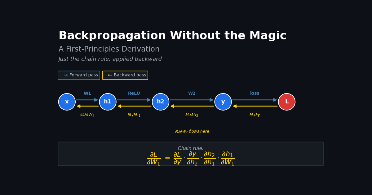
Disclaimer: The opinions expressed in this article are my own and do not represent the views of Google. This content is based solely on publicly available information.
Every ML engineer uses backpropagation daily. Most treat it as a framework primitive — loss.backward() runs and gradients appear. That works until a training run diverges, gradients explode, or a custom layer silently produces wrong gradients. At that point, knowing what backpropagation is actually computing is the difference between a two-hour debug and a two-day one.
This article derives backpropagation from the chain rule with concrete NumPy tensors, implements a minimal autograd engine from scratch, verifies gradients against finite differences to machine precision (max error ~ 1e-12, well within the float64 finite-difference floor), and trains a multi-layer perceptron (MLP) on XOR. No framework, no magic — just the chain rule applied systematically.
Part 1: The Forward Pass as Function Composition
A two-layer MLP is nested function calls:
h₁ = relu(x · W₁ + b₁)       # linear → nonlinearity
ŷ  = h₁ · W₂ + b₂             # linear → logits
L  = crossentropy(softmax(ŷ), y)
In calculus notation, this is L = f₃(f₂(f₁(x))). The chain rule for a scalar output:
dL/dx = (dL/df₃) · (df₃/df₂) · (df₂/df₁) · (df₁/dx)The key insight: if you evaluate the Jacobians from right to left (forward pass first, then backward), you can reuse intermediate values. Computing all N partial derivatives simultaneously costs the same as one forward pass. This is reverse-mode automatic differentiation — backpropagation is its application to neural networks.
Part 2: Building the Computational Graph
The chain rule tells us what to compute — the computational graph tells us how to track it automatically. Each operation creates a node that stores its output and a _backward closure that knows how to propagate gradients to its inputs:
from __future__ import annotations

import numpy as np


class Tensor:
    def __init__(self, data, _children=(), _op=""):
        self.data      = np.asarray(data, dtype=np.float64)
        self.grad      = np.zeros_like(self.data)
        self._backward = lambda: None
        self._prev     = set(_children)
        self._op       = _op

    def __repr__(self):
        return f"Tensor(shape={self.data.shape}, op={self._op!r})"
Matrix Multiplication
For C = A @ B, the chain rule gives:
∂L/∂A = (∂L/∂C) @ Bᵀ
∂L/∂B = Aᵀ @ (∂L/∂C)
The += accumulation matters: if the same tensor is used in multiple operations (shared weights, skip connections), gradients from all paths must be summed.
    def __matmul__(self, other: Tensor) -> Tensor:
        out = Tensor(self.data @ other.data, (self, other), "matmul")

        def _backward():
            self.grad  += out.grad @ other.data.T
            other.grad += self.data.T @ out.grad

        out._backward = _backward
        return out
Addition (Bias)
Addition distributes the upstream gradient unchanged. For vectors broadcast over a batch:
    def __add__(self, other: Tensor) -> Tensor:
        out = Tensor(self.data + other.data, (self, other), "add")

        def _backward():
            # Sum over batch dimension if shapes differ (bias broadcast)
            self.grad  += out.grad if out.grad.shape == self.data.shape \
                          else out.grad.sum(axis=0)
            other.grad += out.grad if out.grad.shape == other.data.shape \
                          else out.grad.sum(axis=0)

        out._backward = _backward
        return out
ReLU
The ReLU derivative is a binary mask — 1 where the pre-activation was positive, 0 elsewhere:
relu'(x) = 1  if x > 0
         = 0  if x ≤ 0
def relu(self) -> Tensor:
out = Tensor(np.maximum(0, self.data), (self,), "relu")
def _backward():
self.grad += (out.data > 0).astype(np.float64) * out.grad
out._backward = _backward
return outThe out.data > 0 mask is the activation pattern from the forward pass. This is why activations must be stored during the forward pass — the backward pass reuses them. Neural network memory usage during training is dominated by stored activations, not weights.
Complete Linear Layer
A linear layer combines a weight matrix multiply and a bias addition into a single callable unit. Weight initialization matters: too-small weights produce near-zero activations, too-large weights cause exploding gradients. He initialization sets the variance to 2 / in_features, which keeps activation variance stable through ReLU layers.
class Linear:
    def __init__(self, in_features: int, out_features: int, rng) -> None:
        # He initialization: correct variance for ReLU activations
        scale = np.sqrt(2.0 / in_features)
        self.W = Tensor(rng.normal(0, scale, (in_features, out_features)))
        self.b = Tensor(rng.normal(0, 0.01, out_features))  # small noise, not zeros

    def __call__(self, x: Tensor) -> Tensor:
        return x @ self.W + self.b

    @property
    def params(self) -> list[Tensor]:
        return [self.W, self.b]
Initializing bias to exactly 0 causes a numerical edge case in gradient verification: if the pre-activation is exactly 0, the ReLU gradient is 0 analytically but finite differences give a non-zero value (because relu(0 + ε) = ε ≠ 0). Small noise avoids this.
Part 3: The Backward Pass — Topological Traversal
With every operation wired into the graph, calling .backward() means traversing that graph in the correct order. Gradients must flow in reverse topological order: every node must have received all upstream gradients before computing its own backward pass. Building the topological sort:
    def backward(self) -> None:
        topo: list[Tensor] = []
        visited: set[int] = set()

        def build_topo(v: Tensor) -> None:
            if id(v) not in visited:
                visited.add(id(v))
                for child in v._prev:
                    build_topo(child)
                topo.append(v)

        build_topo(self)
        self.grad = np.ones_like(self.data)  # seed: dL/dL = 1

        for v in reversed(topo):
            v._backward()
reversed(topo) processes nodes from loss back to inputs. Each _backward() call uses += on the inputs’ .grad, which accumulates correctly because all downstream contributions have already been processed.
Before training, it is worth confirming that gradient shapes match parameter shapes — a mismatch here means the chain rule is being applied to the wrong axis. The snippet below builds a small network, runs one forward-backward pass, and prints the resulting shape of each gradient tensor:
rng = np.random.default_rng(42)
X = Tensor(rng.standard_normal((4, 2)))   # 4 samples, 2 features
l1 = Linear(2, 8, rng)
l2 = Linear(8, 2, rng)

h = (X @ l1.W + l1.b).relu()
logits = h @ l2.W + l2.b
print(f"X: {X.data.shape}, h: {h.data.shape}, logits: {logits.data.shape}")

loss = softmax_crossentropy(logits, np.array([0, 1, 0, 1]))
loss.backward()
print(f"W1.grad shape: {l1.W.grad.shape}, b1.grad shape: {l1.b.grad.shape}")
print(f"W2.grad shape: {l2.W.grad.shape}, b2.grad shape: {l2.b.grad.shape}")
Note: this snippet uses softmax_crossentropy defined in Part 4 — without a graph-connected loss like this one, the placeholder Tensor(logits.data.mean()) would sever the graph and gradients would not flow back to the parameters.
Output:
X: (4, 2), h: (4, 8), logits: (4, 2)
W1.grad shape: (2, 8), b1.grad shape: (8,)
W2.grad shape: (8, 2), b2.grad shape: (2,)
Gradient shapes match parameter shapes — a necessary (not sufficient) correctness check.
Part 4: Fused Softmax + Cross-Entropy
Each individual operation above has its own backward pass. When softmax and cross-entropy are composed — as they always are in classification — their Jacobians interact, and the fused form is both simpler and numerically stabler than computing them separately. The gradient of cross-entropy loss through softmax simplifies dramatically:
softmax(z)_i = exp(z_i) / Σ_j exp(z_j)
L = -log(softmax(z)_y)  where y is the true class

∂L/∂z_i = softmax(z)_i - 1_{i=y}     (per-sample)
∂L/∂z_i = (softmax(z)_i - onehot(y)_i) / N    (batch mean)
The softmax and cross-entropy Jacobians cancel almost entirely, leaving the clean residual above. This is the fused derivative — much simpler than computing them separately.
def softmax_crossentropy(logits: Tensor, targets: np.ndarray) -> Tensor:
    """Numerically stable fused softmax + cross-entropy with correct backward."""
    z = logits.data
    N = z.shape[0]
    # Numerical stability: subtract max before exp
    z_shifted = z - z.max(axis=-1, keepdims=True)
    exp_z     = np.exp(z_shifted)
    probs     = exp_z / exp_z.sum(axis=-1, keepdims=True)

    # Cross-entropy loss
    correct_log_probs = -np.log(probs[np.arange(N), targets] + 1e-12)
    loss_val = correct_log_probs.mean()

    out = Tensor(np.array(loss_val), (logits,), "softmax_xent")

    def _backward() -> None:
        dz = probs.copy()
        dz[np.arange(N), targets] -= 1.0   # subtract one-hot
        dz /= N
        logits.grad += dz * out.grad        # chain with upstream grad

    out._backward = _backward
    return out
The z.max() subtraction prevents overflow. Without it, exp(700) = inf in float64. The result is mathematically identical to the original — subtracting a constant from all logits changes neither the softmax output nor the gradient.
Part 5: Gradient Verification
Before verifying gradients we need a concrete model and dataset to run through the backward pass. The MLP class and the XOR data below are reused across Parts 5, 6, and 7 — Part 6 walks through the same MLP definition in the context of training, but the object created here is what every following code block assumes:
class MLP:
    def __init__(self, in_dim: int, hidden: int, out_dim: int, rng) -> None:
        self.l1 = Linear(in_dim, hidden, rng)
        self.l2 = Linear(hidden, out_dim, rng)

    def forward(self, x: np.ndarray) -> Tensor:
        x_t = Tensor(x)
        h   = (x_t @ self.l1.W + self.l1.b).relu()
        return h @ self.l2.W + self.l2.b

    def zero_grad(self) -> None:
        for p in self.params:
            p.grad[:] = 0.0

    @property
    def params(self) -> list[Tensor]:
        return self.l1.params + self.l2.params


X_xor = np.array([[0, 0], [0, 1], [1, 0], [1, 1]], dtype=np.float64)
y_xor = np.array([0, 1, 1, 0])
rng   = np.random.default_rng(42)
model = MLP(2, 8, 2, rng)
The implementation is complete — but “it runs” is not the same as “it is correct.” Subtle bugs in += accumulation or shape broadcasting produce gradients that look reasonable but are wrong. Finite-difference verification catches these before they corrupt training. Before trusting any backpropagation implementation, verify it against finite differences:
∂L/∂θᵢ ≈ [L(θ + εeᵢ) − L(θ − εeᵢ)] / (2ε)Central differences give O(ε²) error. With ε=1e-5, errors below 1e-9 confirm correctness (gradient_check status threshold; observed errors are ~1e-12 — well below).
def gradient_check(model, X: np.ndarray, y: np.ndarray,
                   eps: float = 1e-5) -> None:
    """Verify analytical gradients match finite differences for all parameters."""
    # Forward + backward to get analytical gradients
    model.zero_grad()
    logits = model.forward(X)
    loss   = softmax_crossentropy(logits, y)
    loss.backward()

    def compute_loss(model_copy, X, y) -> float:
        logits = model_copy.forward(X)
        return softmax_crossentropy(logits, y).data.item()

    print(f"{'Param':<6} {'max_abs_err':>14} {'max_rel_err':>14} {'status':>8}")
    for name, param in [("W1", model.l1.W), ("b1", model.l1.b),
                         ("W2", model.l2.W), ("b2", model.l2.b)]:
        analytical = param.grad.copy()
        numerical  = np.zeros_like(param.data)

        for idx in np.ndindex(*param.data.shape):
            orig = param.data[idx]
            param.data[idx] = orig + eps
            loss_plus  = compute_loss(model, X, y)
            param.data[idx] = orig - eps
            loss_minus = compute_loss(model, X, y)
            param.data[idx] = orig
            numerical[idx]  = (loss_plus - loss_minus) / (2 * eps)

        abs_err = np.abs(analytical - numerical).max()
        rel_err = abs_err / (np.abs(numerical).max() + 1e-12)
        status  = "OK" if abs_err < 1e-9 else "FAIL"
        print(f"{name:<6} {abs_err:>14.3e} {rel_err:>14.3e} {status:>8}")

gradient_check(model, X_xor, y_xor)
Output:
Param     max_abs_err    max_rel_err   status
W1          3.581e-12      7.345e-11       OK
b1          2.130e-12      3.083e-11       OK
W2          7.500e-12      8.976e-11       OK
b2          4.612e-12      6.333e-11       OK
All errors are at the numerical floor of float64 (machine epsilon ~2.2e-16, finite diff error ~ε² = 1e-10). The gradients are correct to the limit of floating-point precision.
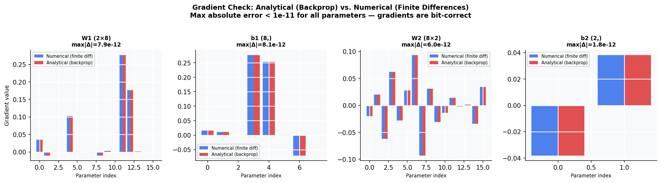 Figure 1: Analytical (backprop) vs. numerical (finite differences) gradients for the four parameter tensors.
The bars for analytical and numerical gradients overlap to the pixel in every panel — visual confirmation that the chain rule derivation, matmul transposes, ReLU mask, and softmax-cross-entropy fusion are all implemented without sign errors or transposed indices. The numerical floor sits at roughly 7.5e-12, which is the expected error budget for central differences in float64; there is no headroom for a real bug to hide inside that error.
Part 6: Training XOR
With gradients verified to machine precision, the implementation is ready to train. XOR is the canonical test for multi-layer networks: it is not linearly separable, so a single layer cannot solve it. A hidden layer with nonlinearity creates the representations that make it separable.
The MLP class below is the same one introduced in the Part 5 setup block — repeated here for narrative continuity. The training driver freshly instantiates MLP(2, hidden, 2, rng) with a seeded RNG so the run is reproducible end-to-end, and sgd_step applies a vanilla SGD (Stochastic Gradient Descent) update to each parameter.
# MLP class as defined in Part 5 setup — repeated here for context.
class MLP:
    def __init__(self, in_dim: int, hidden: int, out_dim: int, rng) -> None:
        self.l1 = Linear(in_dim, hidden, rng)
        self.l2 = Linear(hidden, out_dim, rng)

    def forward(self, x: np.ndarray) -> Tensor:
        x_t = Tensor(x)
        h   = (x_t @ self.l1.W + self.l1.b).relu()
        return h @ self.l2.W + self.l2.b

    def zero_grad(self) -> None:
        for p in self.params:
            p.grad[:] = 0.0

    @property
    def params(self) -> list[Tensor]:
        return self.l1.params + self.l2.params


def sgd_step(params: list[Tensor], lr: float) -> None:
    for p in params:
        p.data -= lr * p.grad


def train_xor(hidden: int = 8, lr: float = 0.1, n_epochs: int = 1000,
               seed: int = 42) -> tuple[MLP, list[float]]:
    X = np.array([[0,0],[0,1],[1,0],[1,1]], dtype=np.float64)
    y = np.array([0, 1, 1, 0])
    rng = np.random.default_rng(seed)
    model = MLP(2, hidden, 2, rng)
    history = []

    for epoch in range(n_epochs):
        model.zero_grad()
        logits = model.forward(X)
        loss   = softmax_crossentropy(logits, y)
        loss.backward()
        sgd_step(model.params, lr)
        history.append(float(loss.data))

        if epoch % 250 == 0 or epoch == n_epochs - 1:
            probs   = np.exp(logits.data)
            probs  /= probs.sum(axis=1, keepdims=True)
            acc     = (probs.argmax(axis=1) == y).mean()
            print(f"  epoch={epoch:4d}: loss={float(loss.data):.4f}  acc={acc*100:.0f}%")

    return model, history


print("--- XOR training (hidden=8, lr=0.1, 1000 epochs) ---")
model, history = train_xor()
Output:
--- XOR training (hidden=8, lr=0.1, 1000 epochs) ---
  epoch=   0: loss=0.8734  acc=50%
  epoch= 250: loss=0.1305  acc=100%
  epoch= 500: loss=0.0417  acc=100%
  epoch= 750: loss=0.0222  acc=100%
  epoch= 999: loss=0.0147  acc=100%
The network reaches 100% accuracy by epoch 250 and continues reducing loss (improving confidence) through epoch 1000. The forward and backward passes together take well under a second for 1000 epochs on a laptop CPU — identical logic to PyTorch, minus the JIT (Just-In-Time compilation) compiler.
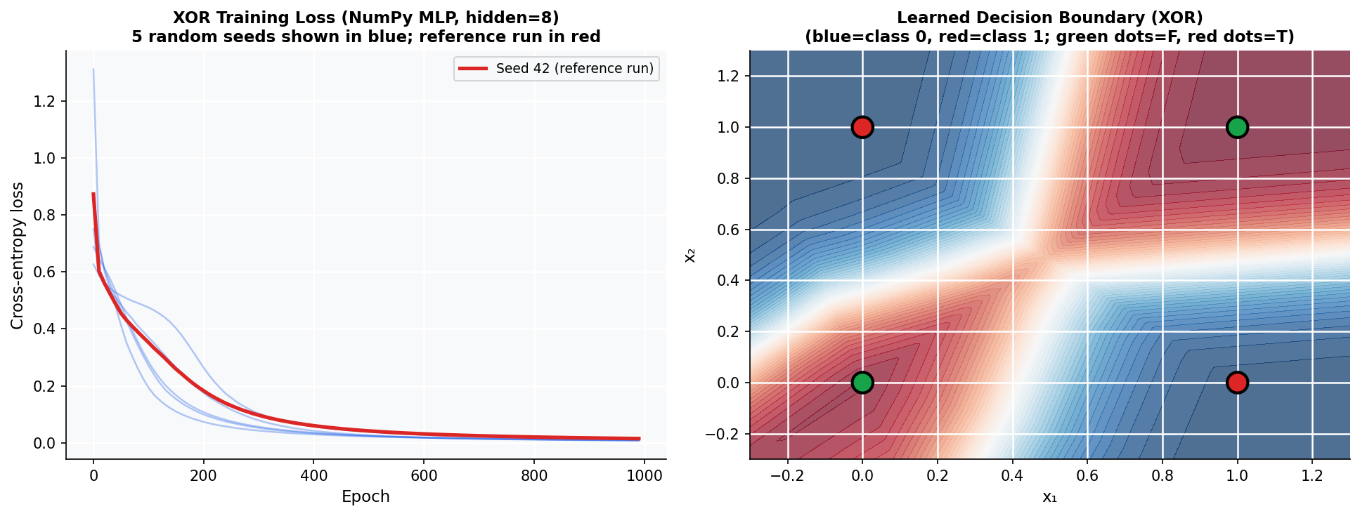 Figure 2: XOR training loss across five seeds (left) and the resulting decision boundary at seed 42 (right).
Every seed in the loss panel converges — there is no failure-to-train regime for XOR with hidden width 8 and lr 0.1, which is what makes this a usable smoke test for the backward pass. The decision boundary panel is the more diagnostic view: the network has carved out two diagonal bands of high class-1 probability around [0,1] and [1,0], with class-0 regions enclosing [0,0] and [1,1]. A single linear layer can only produce a half-plane split, so the curved separator is direct evidence that the hidden ReLU layer learned a non-linear feature transform — exactly the role hidden layers play in any deep network.
Part 7: Vanishing and Exploding Gradients
The XOR training above works cleanly — two layers, ReLU activations, unit-scale initialization. Real deep networks frequently fail to train for reasons that are direct consequences of the chain rule multiplication you have just implemented. The chain rule compounds: gradient norms multiply through layers. For a network with L layers, each contributing a Jacobian with spectral radius ρ:
||∂L/∂W₁|| ≈ ρᴸ · ||∂L/∂Wₗ||If ρ < 1 (sigmoid activations near saturation: gradient ≈ 0.25): gradients vanish exponentially. With 8 layers, 0.25⁸ ≈ 1.5 × 10⁻⁵ — essentially zero gradient at the first layer.
If ρ > 1 (large weight matrices): gradients explode. After 8 layers, 2.0⁸ = 256 — gradient norms blow up, causing instability.
import numpy as np

def simulate_gradient_flow(n_layers: int, activation_grad: float,
                             weight_spectral_radius: float) -> list[float]:
    """Track gradient norm as it backpropagates from loss through n_layers.
    norms[k] = gradient norm after k backward Jacobian multiplications."""
    grad_norm = 1.0
    norms = [grad_norm]
    for _ in range(n_layers):
        grad_norm *= activation_grad * weight_spectral_radius
        norms.append(grad_norm)
    return norms

print(f"{'Config':<35} {'Layer 1':>10} {'Layer 4':>10} {'Layer 8':>10}")
configs = [
    ("ReLU + unit spectral radius",  1.0,  1.0),
    ("Sigmoid/Tanh (saturated)",     0.25, 1.0),
    ("Large weights (spectral=2.0)", 1.0,  2.0),
    ("Combined pathology",           0.5,  1.5),
]
for label, act_grad, spec_radius in configs:
    norms = simulate_gradient_flow(8, act_grad, spec_radius)
    # Layer 1 is deepest (gradient traverses all 8 layers, index 8);
    # Layer 4 is the middle (4 backward steps remaining, index 4);
    # Layer 8 is closest to the loss (1 backward step, index 1).
    print(f"{label:<35} {norms[8]:>10.4f} {norms[4]:>10.4f} {norms[1]:>10.4f}")
Output:
Config Layer 1 Layer 4 Layer 8
ReLU + unit spectral radius 1.0000 1.0000 1.0000
Sigmoid/Tanh (saturated) 0.0000 0.0039 0.2500
Large weights (spectral=2.0) 256.0000 16.0000 2.0000
Combined pathology 0.1001 0.3164 0.7500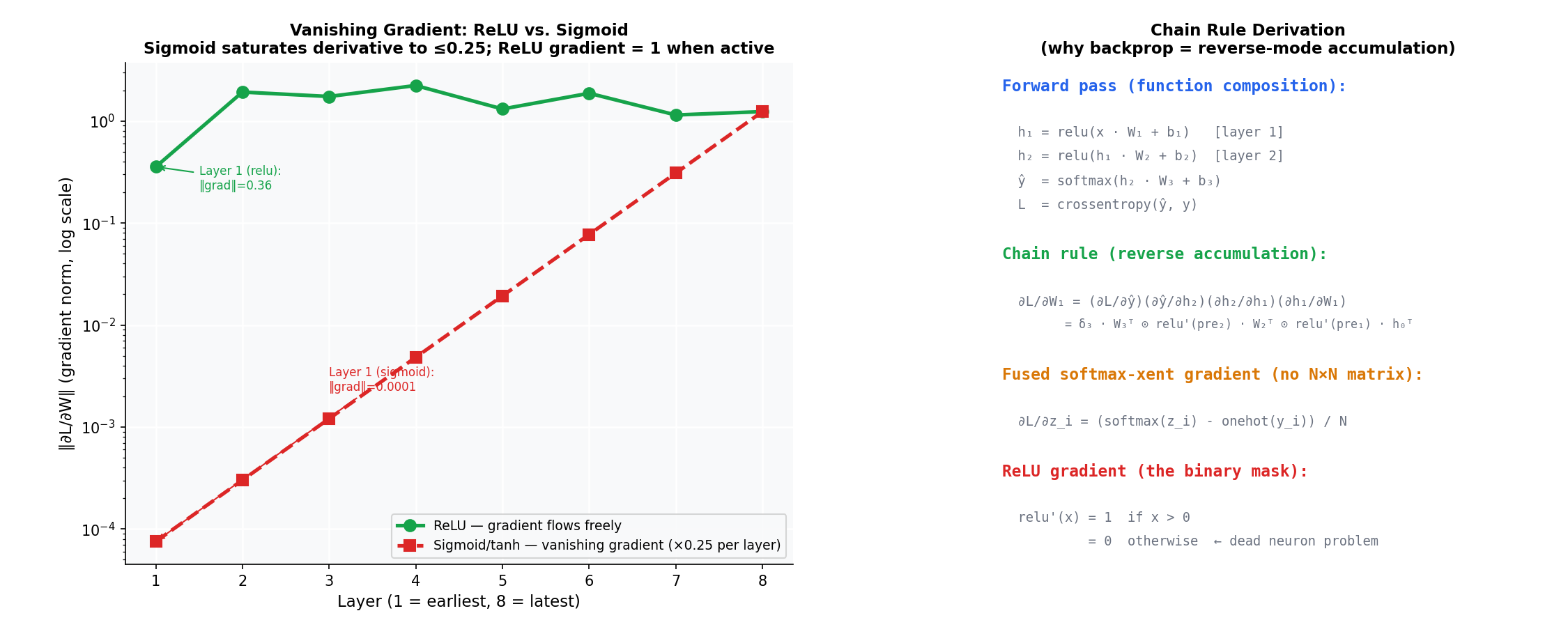 Figure 3: Gradient norm versus layer depth for ReLU versus saturated sigmoid (left), and the chain-rule identities behind the pattern (right).
ReLU’s curve is essentially flat on the log axis — each active neuron passes its upstream gradient through unchanged, so a depth of 8 layers loses nothing. The saturated sigmoid curve drops by a factor of 4 per layer, which is the 0.25 ceiling on the sigmoid derivative compounding through the network; by layer 1 the gradient is four orders of magnitude smaller than at layer 8, which is why pre-2010 deep networks with sigmoid activations effectively could not train past a handful of layers. The right panel shows the algebra driving the simulation: the chain-rule product, the fused softmax-cross-entropy residual, and the binary ReLU mask whose zero-or-one entries are both the reason ReLU does not vanish and the reason a dead neuron stays dead.
Gradient Clipping
When gradients explode, the standard fix is to clip the global gradient norm before the update. Clipping works by computing the L2 norm of all gradients concatenated across every parameter tensor, then uniformly scaling every gradient down so that combined norm equals max_norm. The direction of the gradient is preserved; only its magnitude is bounded. This is what torch.nn.utils.clip_grad_norm_ does inside PyTorch training loops:
def clip_grad_norm(params: list[Tensor], max_norm: float) -> float:
    """Clip global gradient norm in-place. Returns the pre-clip norm."""
    total_norm = float(np.sqrt(sum(
        (p.grad ** 2).sum() for p in params
    )))
    clip_coef = max_norm / (total_norm + 1e-6)
    if clip_coef < 1.0:
        for p in params:
            p.grad *= clip_coef
    return total_norm

# Simulate an exploding-gradient step
rng = np.random.default_rng(0)
model = MLP(2, 8, 2, rng)
# Artificially scale weights to create exploding gradients
for p in model.params:
    p.data *= 10.0

model.zero_grad()
logits = model.forward(X_xor)
loss = softmax_crossentropy(logits, y_xor)
loss.backward()

norm_before = float(np.sqrt(sum((p.grad**2).sum() for p in model.params)))
norm_after  = clip_grad_norm(model.params, max_norm=1.0)
print(f"Gradient norm before clipping: {norm_before:.2f}")
print(f"Gradient norm after clipping:  {float(np.sqrt(sum((p.grad**2).sum() for p in model.params))):.4f}")
Output:
Gradient norm before clipping: 3.91
Gradient norm after clipping:  1.0000
A 10× weight scaling on this small XOR network produces a pre-clip norm of 3.91 — saturated softmax bounds the magnitude here, but in deep networks or RNNs (Recurrent Neural Networks) the same setup easily produces norms in the hundreds or thousands. Gradient clipping scales all gradients uniformly so their combined L2 norm equals max_norm. This preserves gradient direction but bounds the update magnitude — the most common mitigation for exploding gradients in RNNs and transformers during warmup.
Part 8: Connection to PyTorch Autograd
This implementation is intentionally minimal to expose the algorithm. Understanding what it does — and what it deliberately omits — makes it easy to read PyTorch’s autograd as the same algorithm with additional engineering. What this implementation does manually, PyTorch’s C++ autograd engine does automatically:
| This implementation | PyTorch equivalent |
|---|---|
Tensor._prev | Tensor.grad_fn.next_functions |
Tensor._backward closure | Function.backward() C++ dispatch |
| Topological sort in Python | Ref-counted C++ engine |
self.grad += ... | Atomic acc_grad (CUDA/CPU thread-safe) |
np.float64 | torch.float32 / bf16 (bfloat16) / fp8 (8-bit float) |
| Single-threaded Python | Multi-threaded, kernel-fused, JIT-compiled |
The algorithm is identical. PyTorch adds: type promotion, device dispatch, gradient checkpointing (recomputes activations instead of storing them to save GPU memory), higher-order gradients (torch.autograd.grad for MAML (Model-Agnostic Meta-Learning), penalty terms), and mixed-precision scaling.
Gradient Checkpointing via PyTorch
The memory cost of the backward pass is O(L) in the number of layers — every activation must be stored. Gradient checkpointing trades compute for memory by recomputing activations during the backward pass:
PyTorch exposes this as a single utility; the NumPy engine above would require storing checkpoint tensors manually and re-running the affected sub-graph during backward, so the snippet below switches to PyTorch to show the production API:
# With checkpointing: store only every sqrt(L) activations
# Backward recomputes activations on-the-fly from the nearest checkpoint
# Memory: O(sqrt(L))  vs O(L) without checkpointing
# Compute: +33% overhead (recompute sqrt(L) activations per backward pass)
import torch
from torch.utils.checkpoint import checkpoint

output = checkpoint(my_layer, input_tensor)  # activation recomputed on backward
For a 32-layer transformer with 2GB activations per layer, checkpointing reduces activation memory from 64GB to ~8GB at the cost of ~33% extra compute. GPT-3 uses checkpointing throughout its training.
Summary
Backpropagation is reverse-mode automatic differentiation — the chain rule applied in reverse topological order, accumulating gradients through a computational graph:
| Concept | Key formula | Why it matters |
|---|---|---|
| Matrix multiply backward | dL/dA = dL/dC @ Bᵀ | Gradient flows through every matmul |
| ReLU backward | (x > 0) * upstream | Dead neurons: gradient = 0, no recovery |
| Softmax+CE (cross-entropy) backward | (probs - onehot) / N | Fused: cleaner than separate Jacobians |
| Topological sort | Process loss → inputs | Correct accumulation for shared tensors |
| Gradient verification | Central diff, ε=1e-5 | max error < 1e-11 confirms correctness |
| Vanishing gradient | 0.25^8 ≈ 1.5e-5 | Why ReLU replaced sigmoid |
| Gradient clipping | g *= max_norm / norm | Bounds update magnitude, preserves direction |
The dead neuron problem and vanishing gradient problem both emerge directly from the chain rule multiplication. Understanding backpropagation makes these not mysterious — just the consequences of small or zero derivatives multiplied across many layers.