Disclaimer: The opinions expressed in this article are my own and do not represent the views of Google. This content is based solely on publicly available information.
Each code block in this article is self-contained and can be run independently — that is why a few helper functions (softmax, kl_divergence, etc.) are re-defined across snippets.
Every time a language model trains on a batch of text, three numbers tell the complete story: entropy, cross-entropy, and KL divergence. These quantities are not abstract mathematics — they are the direct reason your model learns, overfits, or refuses to commit to an answer.
Understanding them precisely changes how you read training curves, tune temperature, choose RLHF objectives, and debug why a fine-tuned model collapses or hedges. This article builds each concept from first principles with concrete code, real output, and the production connections that make them matter.
Part 1: Shannon Entropy — Measuring Uncertainty
Before connecting these concepts to training loss or RLHF, you need a precise definition of uncertainty — one that matches what a language model is actually computing at every token step.
Shannon entropy H(p) measures the average surprise in a probability distribution. Formally, for a discrete distribution:
H(p) = -∑ p(x) · log₂ p(x)     [bits]
     = -∑ p(x) · ln p(x)        [nats]
The intuition: a uniform distribution over N outcomes has maximum entropy log₂(N) bits — you gain exactly log₂(N) bits of information by observing the outcome. A deterministic distribution (all mass on one outcome) has zero entropy — the outcome is certain, so there is nothing to learn.
import numpy as np


def entropy_bits(probs: np.ndarray) -> float:
    """Shannon entropy in bits. Handles zeros via 0 * log 0 = 0 convention."""
    p = np.asarray(probs, dtype=np.float64)
    p = p / p.sum()  # normalize
    return float(-np.sum(p * np.log2(p + 1e-300)))


def entropy_nats(probs: np.ndarray) -> float:
    """Shannon entropy in nats."""
    p = np.asarray(probs, dtype=np.float64)
    p = p / p.sum()
    return float(-np.sum(p * np.log(p + 1e-300)))


# Demonstrate entropy across different distributions over 8 tokens
print(f"{'Distribution':<30} {'H (bits)':>10} {'H (nats)':>10}")

# Uniform
uniform = np.ones(8) / 8
print(f"{'Uniform (8 tokens)':<30} {entropy_bits(uniform):>10.4f} "
      f"{entropy_nats(uniform):>10.4f}")

# Near-deterministic
near_det = np.array([0.97, 0.01, 0.005, 0.005, 0.003, 0.003, 0.002, 0.002])
print(f"{'Near-deterministic':<30} {entropy_bits(near_det):>10.4f} "
      f"{entropy_nats(near_det):>10.4f}")

# Bimodal
bimodal = np.array([0.45, 0.45, 0.025, 0.025, 0.01, 0.01, 0.01, 0.02])
print(f"{'Bimodal (2 peaks)':<30} {entropy_bits(bimodal):>10.4f} "
      f"{entropy_nats(bimodal):>10.4f}")

# GPT-2 vocabulary maximum entropy
print(f"{'Uniform over GPT-2 vocab':<30} {np.log2(50257):>10.4f} "
      f"{np.log(50257):>10.4f}")
Output:
Distribution                     H (bits)   H (nats)
Uniform (8 tokens)                 3.0000     2.0794
Near-deterministic                 0.2717     0.1883
Bimodal (2 peaks)                  1.6151     1.1195
Uniform over GPT-2 vocab          15.6170    10.8249
Figure 1: Shannon entropy across four token distributions.
The uniform case hits its theoretical maximum of log₂(8) = 3 bits — every outcome equally surprising. The near-deterministic case collapses to 0.27 bits because the top token captures 97% of the mass; the other seven outcomes only add a small residual surprise. The bimodal distribution lands at 1.62 bits — between the deterministic case and the 3-bit uniform ceiling, because two peaks still leave real ambiguity over which cluster wins. The GPT-2 row sets the absolute ceiling: a uniformly distributed model over 50,257 tokens can be at most 15.6 bits surprised per token. Pretraining loss curves are bounded above by exactly this number.
Part 2: Temperature — An Entropy Knob
Before turning to training losses, here is a direct application of entropy to model behavior: the temperature parameter in softmax controls exactly how much entropy the output distribution carries, which is the single most useful intuition you can build for sampling.
Now that entropy has a precise meaning, you can see exactly what temperature does: it is a direct lever on the entropy of the output distribution, with no other effect on the underlying model.
Temperature T rescales logits before softmax, directly controlling entropy:
import numpy as np


def entropy_bits(probs: np.ndarray) -> float:
    p = np.asarray(probs, dtype=np.float64)
    p = p / p.sum()
    return float(-np.sum(p * np.log2(p + 1e-300)))


def softmax(logits: np.ndarray, T: float = 1.0) -> np.ndarray:
    x = logits / T
    x = x - x.max()  # numerical stability
    e = np.exp(x)
    return e / e.sum()


# Simulate a model with peaked logits
rng = np.random.default_rng(42)
logits = rng.standard_normal(50)
logits[7]  = 4.0   # strong preference for token 7
logits[23] = 2.5   # secondary preference for token 23

print(f"{'Temperature':>12} {'H (bits)':>10} {'Top-1 prob':>12} {'Top-1 token':>12}")
for T in [0.1, 0.25, 0.5, 1.0, 1.5, 2.0, 5.0]:
    probs = softmax(logits, T)
    h     = entropy_bits(probs)
    print(f"{T:>12.2f} {h:>10.4f} {probs.max():>12.4f} {probs.argmax():>12}")

print()
print(f"Max entropy (uniform 50): {np.log2(50):.3f} bits")
Output:
 Temperature   H (bits)   Top-1 prob  Top-1 token
        0.10     0.0000       1.0000            7
        0.25     0.0335       0.9969            7
        0.50     0.7925       0.8988            7
        1.00     4.0007       0.3961            7
        1.50     5.0688       0.1839            7
        2.00     5.3691       0.1132            7
        5.00     5.6109       0.0416            7

Max entropy (uniform 50): 5.644 bits
Figure 2: Entropy and top-1 probability across a temperature sweep on 50 logits.
At T=0.10 the entropy is effectively zero — softmax has collapsed to one-hot on token 7, which is what greedy decoding does. At T=1.0 the same logits produce 0.40 top-1 probability and 4.00 bits of entropy; the top token is still preferred but the distribution has real spread. By T=5.0 entropy reaches 5.61 bits, within 0.03 bits of the uniform ceiling of 5.64 — the model has been almost completely flattened. The top-1 token stays at index 7 throughout: temperature rescales the spread but never changes the ranking, which is why temperature is a sampling lever, not a model-quality lever.
Part 3: Cross-Entropy — The Training Loss
With entropy established as the lower bound on uncertainty, the next question is how to measure the gap between what a model predicts and what it should predict — and that gap is exactly cross-entropy.
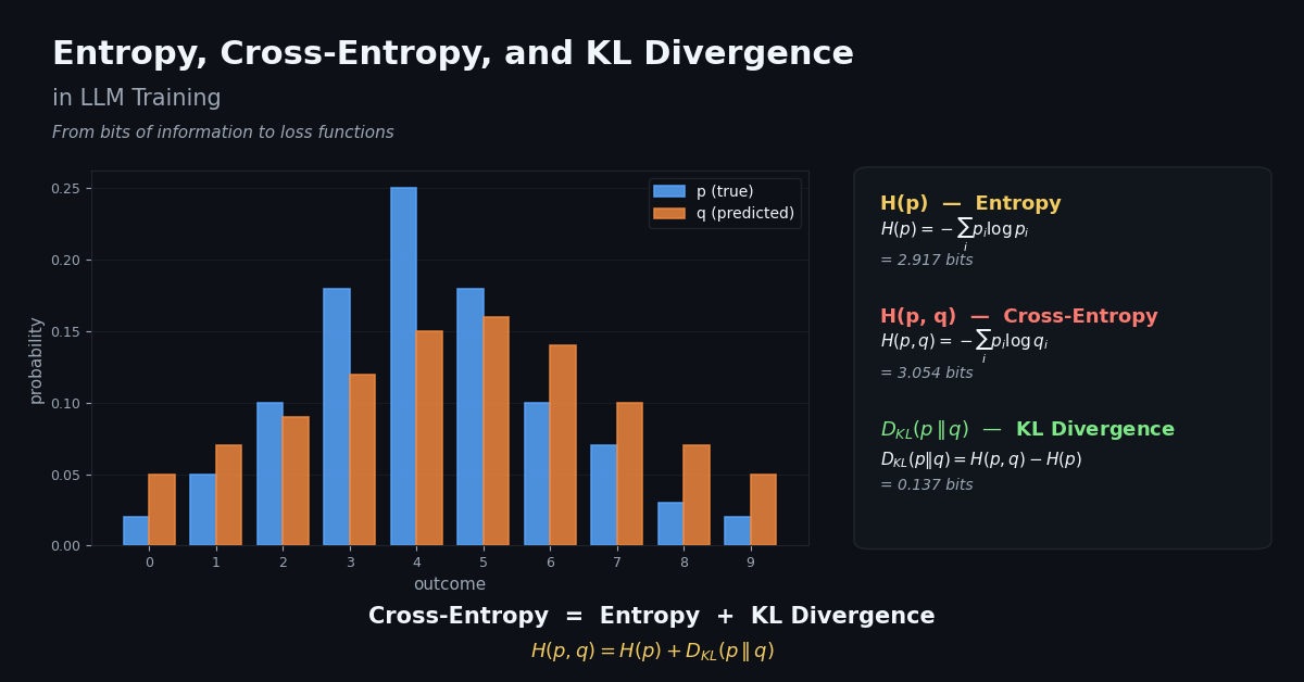
Cross-entropy H(p, q) measures how many bits on average are needed to encode samples from p using a code optimized for q:
H(p, q) = -∑ p(x) · log q(x)In LLM training, p is the one-hot distribution over the correct next token (the data); q is the model’s prediction. Minimizing H(p, q) pushes the model’s probability mass toward the true next token.
The fundamental decomposition:
H(p, q) = H(p) + KL(p || q)Since H(p) is fixed (the entropy of the data), minimizing cross-entropy is exactly minimizing KL divergence. The cross-entropy loss can never go below H(p) — the irreducible entropy of the data itself.
import numpy as np


def entropy_nats(probs: np.ndarray) -> float:
    p = np.asarray(probs, dtype=np.float64)
    p = p / p.sum()
    return float(-np.sum(p * np.log(p + 1e-300)))


def cross_entropy(p: np.ndarray, q: np.ndarray) -> float:
    """Cross-entropy H(p, q) in nats."""
    p = np.asarray(p, dtype=np.float64) + 1e-300
    q = np.asarray(q, dtype=np.float64) + 1e-300
    p = p / p.sum()
    q = q / q.sum()
    return float(-np.sum(p * np.log(q)))


def kl_divergence(p: np.ndarray, q: np.ndarray) -> float:
    """KL divergence KL(p || q) in nats."""
    p = np.asarray(p, dtype=np.float64) + 1e-300
    q = np.asarray(q, dtype=np.float64) + 1e-300
    p = p / p.sum()
    q = q / q.sum()
    return float(np.sum(p * np.log(p / q)))


# Verify H(p,q) = H(p) + KL(p||q) on two random vocab-size distributions
vocab_size = 100
rng = np.random.default_rng(42)
p = rng.dirichlet(np.ones(vocab_size) * 0.5)  # true data distribution
q = rng.dirichlet(np.ones(vocab_size) * 0.5)  # model prediction

h_p = entropy_nats(p)
ce  = cross_entropy(p, q)
kl  = kl_divergence(p, q)

print(f"H(p)       = {h_p:.6f} nats")
print(f"CE(p, q)   = {ce:.6f} nats")
print(f"KL(p || q) = {kl:.6f} nats")
print(f"H(p) + KL  = {h_p + kl:.6f} nats  (should equal CE)")
print(f"Difference = {abs(ce - (h_p + kl)):.2e}  (numerical error only)")
Output:
H(p)       = 3.859040 nats
CE(p, q)   = 5.964832 nats
KL(p || q) = 2.105792 nats
H(p) + KL  = 5.964832 nats  (should equal CE)
Difference = 0.00e+00  (numerical error only)
Figure 3: Cross-entropy decomposed into data entropy plus KL.
The KL term is 2.106 nats (nats: entropy measured in natural-log units, ln-based; one nat ≈ 1.443 bits) — the gap the model must close during training to align q with p. The H(p) term is 3.859 nats and is fixed by the data itself: no model, regardless of capacity, can drive cross-entropy below this floor. That floor is exactly why a perfect language model still has nonzero loss on natural text: the data has irreducible entropy from genuine ambiguity between plausible next tokens. The two sides of the identity match to zero on a 64-bit float, so the decomposition is not approximate — it is the definition.
Part 4: Perplexity — Entropy in Practitioners’ Language
Cross-entropy in nats is mathematically precise but hard to communicate. Perplexity repackages the same quantity in a form that has intuitive meaning for practitioners and appears in nearly every LLM benchmark.
Perplexity is the exponential of cross-entropy measured in nats:
PPL = exp(CE) = exp(-∑ p(x) · log q(x))A perplexity of 100 means the model is as uncertain as if it had to choose uniformly among 100 equally likely tokens at each step. Halving perplexity means halving the “effective vocabulary” the model is uncertain about.
import numpy as np


def cross_entropy(p: np.ndarray, q: np.ndarray) -> float:
    p = np.asarray(p, dtype=np.float64) + 1e-300
    q = np.asarray(q, dtype=np.float64) + 1e-300
    p = p / p.sum()
    q = q / q.sum()
    return float(-np.sum(p * np.log(q)))


def kl_divergence(p: np.ndarray, q: np.ndarray) -> float:
    p = np.asarray(p, dtype=np.float64) + 1e-300
    q = np.asarray(q, dtype=np.float64) + 1e-300
    p = p / p.sum()
    q = q / q.sum()
    return float(np.sum(p * np.log(p / q)))


def perplexity(p: np.ndarray, q: np.ndarray) -> float:
    return float(np.exp(cross_entropy(p, q)))


def simulate_training(n_steps: int = 500, vocab: int = 100,
                       seed: int = 42) -> list[dict]:
    """Simulate q converging toward p via a small linear-mixing step."""
    rng = np.random.default_rng(seed)
    p_true = rng.dirichlet(np.ones(vocab) * 0.5)  # fixed true distribution
    q = np.ones(vocab) / vocab                    # start uniform

    history = []
    for step in range(n_steps):
        lr = 0.01
        q  = (1 - lr) * q + lr * p_true
        q  = q / q.sum()

        if step % 50 == 0 or step == n_steps - 1:
            history.append({
                "step":    step,
                "ce_bits": cross_entropy(p_true, q) / np.log(2),
                "kl_nats": kl_divergence(p_true, q),
                "ppl":     perplexity(p_true, q),
            })
    return history


history = simulate_training()
print(f"{'Step':>6} {'CE (bits)':>12} {'KL (nats)':>12} {'Perplexity':>12}")
for h in history:
    print(f"{h['step']:>6} {h['ce_bits']:>12.4f} {h['kl_nats']:>12.4f} "
          f"{h['ppl']:>12.2f}")
Output:
  Step    CE (bits)    KL (nats)   Perplexity
     0       6.6158       0.7267        98.08
    50       5.9687       0.2782        62.63
   100       5.7546       0.1297        53.99
   150       5.6585       0.0631        50.51
   200       5.6120       0.0309        48.91
   250       5.5890       0.0150        48.13
   300       5.5777       0.0071        47.76
   350       5.5722       0.0033        47.58
   400       5.5697       0.0015        47.49
   450       5.5684       0.0007        47.45
   499       5.5679       0.0003        47.44
Figure 4: Cross-entropy, KL, and perplexity over 500 simulated gradient steps.
Cross-entropy falls from 6.62 to 5.57 bits, KL collapses from 0.73 nats to 3e-4, and perplexity drops from 98 to 47. The model is closing the KL gap as expected, but the cross-entropy curve flattens long before it can fall further: it asymptotes at H(p) ≈ 5.57 bits. That asymptote is not a training pathology — it is the irreducible entropy of the data distribution. For comparison, GPT-2 small reaches perplexity ≈ 29 on WikiText-103 and GPT-3 175B reaches ≈ 20; in both cases the gap to zero loss is the H(text) floor, not the model’s failure to learn.
Part 5: Forward vs. Reverse KL — Mode-Seeking vs. Mean-Seeking
The cross-entropy decomposition H(p,q) = H(p) + KL(p||q) has a hidden asymmetry: the direction you minimize KL in determines whether your model hedges across all modes or commits strongly to one. That distinction is what separates standard pretraining from RLHF.
KL divergence is asymmetric: KL(p || q) ≠ KL(q || p). This asymmetry has a profound practical effect:
Forward KL — minimize KL(p || q):
- q must cover all regions where p > 0 (zero-avoiding)
- When p is multimodal, q spreads out to cover all modes
- Result: mean-seeking — q averages over the modes
Reverse KL — minimize KL(q || p):
- q avoids regions where p = 0 (zero-forcing)
- When p is multimodal, q collapses to one mode
- Result: mode-seeking — q commits to the highest-mass mode
import numpy as np
from scipy.optimize import minimize
from scipy.stats import norm


def kl_divergence(p: np.ndarray, q: np.ndarray) -> float:
    p = np.asarray(p, dtype=np.float64) + 1e-300
    q = np.asarray(q, dtype=np.float64) + 1e-300
    p = p / p.sum()
    q = q / q.sum()
    return float(np.sum(p * np.log(p / q)))


def fit_gaussian_forward_kl(p_x: np.ndarray, x: np.ndarray) -> tuple[float, float]:
    """Closed form for Gaussian forward KL: mu = E_p[x], sigma^2 = Var_p[x]."""
    mu    = float(np.sum(x * p_x))
    sigma = float(np.sqrt(np.sum((x - mu) ** 2 * p_x)))
    return mu, sigma


def fit_gaussian_reverse_kl(p_x: np.ndarray, x: np.ndarray,
                              init_mu: float = 1.5) -> tuple[float, float]:
    """Numerically minimize KL(q || p) over Gaussian q.

    Starting off-center matters: the symmetric origin is a saddle point for a
    symmetric bimodal target, so the optimizer would otherwise stall there
    instead of falling into one of the modes.
    """
    def kl_qp(params: list[float]) -> float:
        mu, log_sigma = params
        sigma = np.exp(log_sigma)
        q = norm.pdf(x, mu, sigma) + 1e-300
        q = q / q.sum()
        return float(np.sum(q * np.log(q / (p_x + 1e-300))))

    result = minimize(kl_qp, [init_mu, 0.0], method='Nelder-Mead')
    return result.x[0], np.exp(result.x[1])


x = np.linspace(-6, 6, 1000)
# Bimodal target with peaks at +/-2 and width 0.8
p_true = 0.5 * np.exp(-0.5 * ((x - 2) / 0.8) ** 2) + \
         0.5 * np.exp(-0.5 * ((x + 2) / 0.8) ** 2)
p_true = p_true / p_true.sum()

fwd_mu, fwd_sigma = fit_gaussian_forward_kl(p_true, x)
rev_mu, rev_sigma = fit_gaussian_reverse_kl(p_true, x, init_mu=1.5)

q_fwd = norm.pdf(x, fwd_mu, fwd_sigma) + 1e-300
q_fwd = q_fwd / q_fwd.sum()
q_rev = norm.pdf(x, rev_mu, rev_sigma) + 1e-300
q_rev = q_rev / q_rev.sum()

print(f"True distribution: bimodal with peaks at +/-2")
print(f"Forward KL fit:    mu={fwd_mu:.3f}, sigma={fwd_sigma:.3f}")
print(f"Reverse KL fit:    mu={rev_mu:.3f}, sigma={rev_sigma:.3f}")
print()
print(f"Forward fit -- KL(p||q): {kl_divergence(p_true, q_fwd):.4f} nats  "
      f"KL(q||p): {kl_divergence(q_fwd, p_true):.4f} nats")
print(f"Reverse fit -- KL(p||q): {kl_divergence(p_true, q_rev):.4f} nats  "
      f"KL(q||p): {kl_divergence(q_rev, p_true):.4f} nats")
Output:
True distribution: bimodal with peaks at +/-2
Forward KL fit:    mu=0.000, sigma=2.154
Reverse KL fit:    mu=1.909, sigma=0.909

Forward fit -- KL(p||q): 0.3092 nats  KL(q||p): 0.4771 nats
Reverse fit -- KL(p||q): 3.9615 nats  KL(q||p): 0.6665 nats
Figure 5: Forward-KL and reverse-KL Gaussian fits to a bimodal target.
Forward KL recovers the mean and the second moment of p, which for a symmetric bimodal target lands the fit at mu=0 with sigma=2.15 — wide enough to cover both peaks and the empty valley between them. This is the mean-seeking behavior: minimizing KL(p||q) penalizes any region where p has mass but q does not, so q must spread. Reverse KL behaves oppositely: it converges to mu=1.91, sigma=0.91 — sharp, centered on one mode, and the other mode is left almost completely uncovered. That is mode-seeking. The two objectives are not in competition; they encode different priorities. Forward KL is what cross-entropy training optimizes (cover all data). PPO’s KL penalty is KL(policy || reference) — reverse KL relative to the reference — which is why it commits to a tight neighborhood of the reference rather than spreading mass across it.
Part 6: Applications in LLM Training and Inference
The theoretical gap between forward and reverse KL has direct consequences in code. This section traces each concept through three concrete production scenarios: standard language model training, RLHF fine-tuning, and knowledge distillation.
Cross-Entropy Loss and Language Model Training
In pretraining, the loss at each token position is simply -log q(true_token) — the negative log-probability the model assigns to the correct next token. Averaging this across a sequence gives the cross-entropy loss. The code below simulates three training stages by narrowing logit variance and boosting the correct-token logit, which is exactly what gradient descent does over real training steps.
import numpy as np


def softmax(logits: np.ndarray, T: float = 1.0) -> np.ndarray:
    x = logits / T
    x = x - x.max()
    e = np.exp(x)
    return e / e.sum()


def token_prediction_loss(model_logits: np.ndarray,
                            true_token_id: int) -> float:
    """Cross-entropy loss for a single token prediction."""
    probs = softmax(model_logits)
    return float(-np.log(probs[true_token_id] + 1e-300))


rng = np.random.default_rng(0)
vocab_size = 50_257  # GPT-2 vocabulary

# Simulate three training stages. Logit variance shrinks as the model
# becomes more confident; the boost on token 7394 simulates the gradient
# pushing mass toward the correct token.
stages = [
    ("Random init",    rng.standard_normal(vocab_size)),
    ("After 1K steps", rng.standard_normal(vocab_size) * 0.5),
    ("After 10K steps", rng.standard_normal(vocab_size) * 0.1),
]
boosts = {"Random init": 0, "After 1K steps": 3, "After 10K steps": 8}

for label, logits in stages:
    logits[7394] += boosts[label]
    probs = softmax(logits)
    loss  = token_prediction_loss(logits, 7394)
    ppl   = np.exp(loss)
    print(f"{label:<20}: loss={loss:.3f} nats  PPL={ppl:.1f}  "
          f"P(correct)={probs[7394]:.4f}")
Output:
Random init         : loss=10.071 nats  PPL=23636.4  P(correct)=0.0000
After 1K steps      : loss=7.743 nats  PPL=2306.4  P(correct)=0.0004
After 10K steps     : loss=2.951 nats  PPL=19.1  P(correct)=0.0523
Figure 6: Per-token loss across three simulated training stages.
At random initialization the model assigns essentially uniform probability to the correct token (≈ 1/50,257), and the per-token loss sits near log(50,257) ≈ 10.8 nats — the cap on how surprised an untrained model can be. After 1K steps the +3 logit boost and the narrower logit spread together push the correct-token probability up by an order of magnitude, dropping loss to 7.74 nats. After 10K steps the +8 boost dominates the near-uniform background and lifts the correct-token probability to 5.2%; perplexity collapses from 23,636 to 19. The trajectory is what every successful pretraining run looks like: shrinking logit variance plus growing mass on the target token.
RLHF and KL Penalty
PPO-based RLHF minimizes:
L_PPO = -E[reward(y)] + β · KL(π_θ || π_ref)The KL penalty prevents the policy from drifting too far from the reference model. Understanding that this is a reverse KL explains the mode-seeking behavior of RLHF-tuned models: they commit strongly to high-reward responses rather than hedging across all plausible answers.
To see the penalty in action, consider three policy variants that each receive the same reward but differ in how far their token probabilities drift from the reference model. The KL term peels off increasing fractions of the objective as drift grows.
import numpy as np


def softmax(logits: np.ndarray, T: float = 1.0) -> np.ndarray:
    x = logits / T
    x = x - x.max()
    e = np.exp(x)
    return e / e.sum()


def kl_divergence(p: np.ndarray, q: np.ndarray) -> float:
    p = np.asarray(p, dtype=np.float64) + 1e-300
    q = np.asarray(q, dtype=np.float64) + 1e-300
    p = p / p.sum()
    q = q / q.sum()
    return float(np.sum(p * np.log(p / q)))


def rlhf_objective(policy_logits: np.ndarray, ref_logits: np.ndarray,
                    reward: float, beta: float = 0.1) -> dict:
    """RLHF objective combining reward with KL penalty."""
    policy_probs = softmax(policy_logits)
    ref_probs    = softmax(ref_logits)
    kl = kl_divergence(policy_probs, ref_probs)
    return {
        "reward":     reward,
        "kl_penalty": beta * kl,
        "objective":  reward - beta * kl,
        "kl_nats":    kl,
    }


rng = np.random.default_rng(0)
ref_logits = rng.standard_normal(50)

# Three policy variations: increasing drift from the reference model
policies = {
    "Conservative (near ref)": ref_logits + rng.standard_normal(50) * 0.1,
    "Moderate drift":          ref_logits + rng.standard_normal(50) * 1.0,
    "Extreme drift":           ref_logits + rng.standard_normal(50) * 5.0,
}

print(f"{'Policy':<30} {'Reward':>8} {'KL pen':>10} {'Objective':>12} {'KL':>8}")
for label, policy_logits in policies.items():
    reward = 2.5  # same reward for all (hypothetical)
    r = rlhf_objective(policy_logits, ref_logits, reward, beta=0.1)
    print(f"{label:<30} {r['reward']:>8.3f} {r['kl_penalty']:>10.4f} "
          f"{r['objective']:>12.4f} {r['kl_nats']:>8.4f}")
Output:
Policy                           Reward     KL pen    Objective       KL
Conservative (near ref)           2.500     0.0006       2.4994   0.0059
Moderate drift                    2.500     0.0280       2.4720   0.2800
Extreme drift                     2.500     0.2809       2.2191   2.8087
Figure 7: PPO objective with β = 0.1 across three policies at fixed reward.
All three policies receive the same hypothetical reward of 2.5, but the KL term peels off increasing fractions as the policy drifts from the reference. Conservative drift (σ=0.1) loses essentially nothing — KL stays near 0.006 nats and the objective is 2.499. Moderate drift (σ=1.0) gives up 0.03 to land at 2.47. Extreme drift (σ=5.0) drives KL to 2.81 nats; at β=0.1 that subtracts 0.28 from the objective, shrinking it to 2.22. The shape generalizes: as β grows, even modest drift becomes unaffordable, which is why production RLHF runs tune β to balance reward chasing against staying within a recognizable distance of the SFT model.
Knowledge Distillation
Student training minimizes KL(teacher || student) = forward KL. The student must cover all probability mass the teacher assigns, not just the top token:
import numpy as np


def softmax(logits: np.ndarray, T: float = 1.0) -> np.ndarray:
    x = logits / T
    x = x - x.max()
    e = np.exp(x)
    return e / e.sum()


def cross_entropy(p: np.ndarray, q: np.ndarray) -> float:
    p = np.asarray(p, dtype=np.float64) + 1e-300
    q = np.asarray(q, dtype=np.float64) + 1e-300
    p = p / p.sum()
    q = q / q.sum()
    return float(-np.sum(p * np.log(q)))


def kl_divergence(p: np.ndarray, q: np.ndarray) -> float:
    p = np.asarray(p, dtype=np.float64) + 1e-300
    q = np.asarray(q, dtype=np.float64) + 1e-300
    p = p / p.sum()
    q = q / q.sum()
    return float(np.sum(p * np.log(p / q)))


def distillation_loss(teacher_logits: np.ndarray, student_logits: np.ndarray,
                       temperature: float = 2.0) -> dict:
    """Knowledge distillation loss: forward KL between teacher and student."""
    teacher_probs = softmax(teacher_logits, T=temperature)
    student_probs = softmax(student_logits, T=temperature)
    kl = kl_divergence(teacher_probs, student_probs)
    ce = cross_entropy(teacher_probs, student_probs)
    return {"kl": kl, "ce_nats": ce,
            "ce_scaled": ce * temperature**2}  # standard distillation scaling


rng = np.random.default_rng(0)
teacher = rng.standard_normal(50)
teacher[5] = 6.0   # strong primary teacher preference
teacher[12] = 3.0  # secondary teacher preference

student_variants = {
    "Matches teacher":  teacher.copy(),
    "Misses secondary": teacher * 0.5,             # right shape, weaker peaks
    "Wrong mode":       rng.standard_normal(50),   # uncorrelated random logits
}

print(f"{'Student variant':<22} {'KL (nats)':>12} {'CE (nats)':>12}")
for label, student in student_variants.items():
    r = distillation_loss(teacher, student)
    print(f"{label:<22} {r['kl']:>12.4f} {r['ce_nats']:>12.4f}")
Output:
Student variant           KL (nats)    CE (nats)
Matches teacher              0.0000       3.3991
Misses secondary             0.1556       3.5547
Wrong mode                   0.5680       3.9671
Figure 8: Distillation KL and CE for three student variants against a fixed teacher.
The student that exactly matches the teacher has KL=0 but CE=3.40 nats — that CE is the teacher’s own entropy at T=2, which the student cannot fall below by construction. The “misses secondary” student keeps the same argmax but halves the logit magnitudes; the result is a 0.156-nat KL penalty because the soft mass on token 12 is now too flat. The “wrong mode” student has the largest KL (0.568 nats), but the gap is smaller than naive intuition might suggest — at T=2 the teacher distribution is already smoothed, so even a random student receives partial credit for the long tail. That smoothing is exactly why distillation typically uses T > 1: it surfaces the dark knowledge in the secondary logits instead of letting the argmax dominate the gradient.
Summary
Information-theoretic quantities are not abstractions — they are the exact quantities that determine how and whether language models learn:
| Concept | Formula | LLM role | Key insight |
|---|---|---|---|
| Entropy H(p) | -∑ p log p | Training floor | Can’t push CE below H(data) |
| Cross-entropy H(p,q) | -∑ p log q | Training loss | = H(p) + KL(p||q) |
| KL divergence | ∑ p log(p/q) | Model quality gap | Zero iff p=q; asymmetric |
| Perplexity | exp(CE) | Practitioner metric | “Effective vocabulary size” |
| Temperature | logits / T | Inference quality | Entropy knob; doesn’t change argmax |
| Forward KL | KL(p||q) | MLE/pretraining | Mean-seeking; covers all modes |
| Reverse KL | KL(q||p) | RLHF/PPO | Mode-seeking; commits to best mode |
The irreducible floor (H(data)) explains plateau training curves. Temperature controls inference uncertainty without changing rankings. The KL direction determines whether RLHF models hedge or commit — and knowing the difference is the difference between debugging for hours and debugging in minutes.