Disclaimer: The opinions expressed in this article are my own and do not represent the views of Google. This content is based solely on publicly available information.
A recommendation model that performs well offline but degrades in production is one of the most common and most expensive problems in machine learning. The gap between training and serving performance — training-serving skew — rarely comes from model architecture. It almost always comes from features.
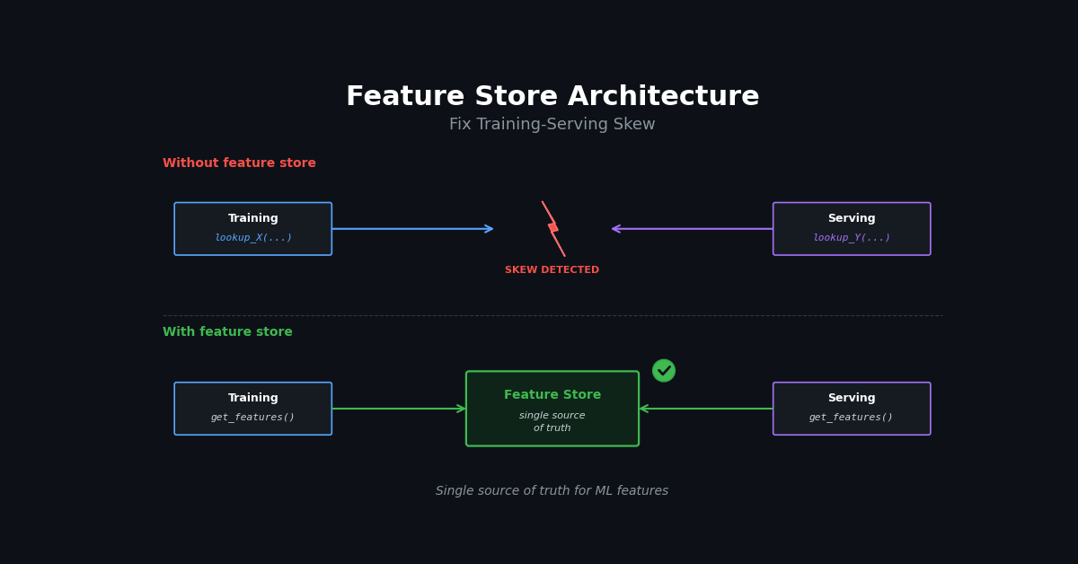
Feature stores exist to solve this problem. A feature store is a system that manages the lifecycle of features: computing them, storing them in a way that enables both historical (training) and real-time (serving) access, and ensuring that the feature computation logic is shared between the two paths. The pattern has been productionised by Uber’s Michelangelo Palette, Airbnb’s Zipline, and the open-source projects that followed (Feast, Tecton, Hopsworks, Databricks Feature Store) — but the underlying primitive is the same: an offline store for historical time-series access, an online store for low-latency lookup, and a single transformation that materialises into both (that is, the same computation writes feature values into both stores, keeping training and serving in sync).
This article explains the core problem (training-serving skew), the architecture that solves it (dual-store with point-in-time joins), and the engineering tradeoffs in feature freshness, latency, and consistency.
The magnitude of the problem is larger than most teams expect. On a synthetic dataset of 50 users and 1,000 training events, a naive join inflates the mean activity_score feature (a continuous user-level engagement signal in [0,1], refreshed every 6 hours per user, with a small upward daily drift) from 0.609 (point-in-time correct) to 0.750 — a +0.141 absolute shift, or 23% upward. A threshold rule applied at 0.5 on the feature value pushes precision down from 0.741 to 0.652 (-0.09) while recall jumps from 0.809 to 0.918 (+0.11): the leaky model over-fires because every example looks more “active” than it really was at event time. F1 drops only 0.011, which is exactly why the bug survives offline evaluation and only surfaces in production telemetry.
The Training-Serving Skew Problem
The 23% feature inflation above is not an edge case — it is the predictable result of a join that ignores event timing, and understanding exactly how it happens is the first step toward fixing it.
Consider a user engagement model that uses a feature called activity_score: a continuous engagement signal in [0,1], refreshed every few hours per user. During training, you have a dataset of (user, event) pairs with labels (did the user click?). Naively, you join each event to the latest available activity_score for that user.
The bug: the “latest available” value at join time was often computed after the event. If you’re training on January 15th data and you join it to activity scores computed on January 30th, you’re using future information as a feature. The feature column in the training set is now a leaky proxy for the label, because both were partly determined by user behaviour between Jan 15 and Jan 30.
This is label leakage in its most common form. The model learns that high activity scores predict clicks — which is true — but during serving, the model sees activity scores computed in real-time (not the future). The distribution of features at serving time is systematically lower than the distribution at training time. The result is degraded offline-to-online transfer: a model that scored well on the held-out test set fires too often and at the wrong moments once it sees real serving-time features.
The simulation (seed 42, 50 synthetic users, 1,000 events over 30 days, feature update every 6 hours per user) reveals the shape of the distortion before the headline numbers. Figure 1 plots the feature value distributions for both join strategies across the same 1,000 events. (Simulation parameters, label-generation rule, and metric computation are spelled out in the Methodology section that follows the metric table.)
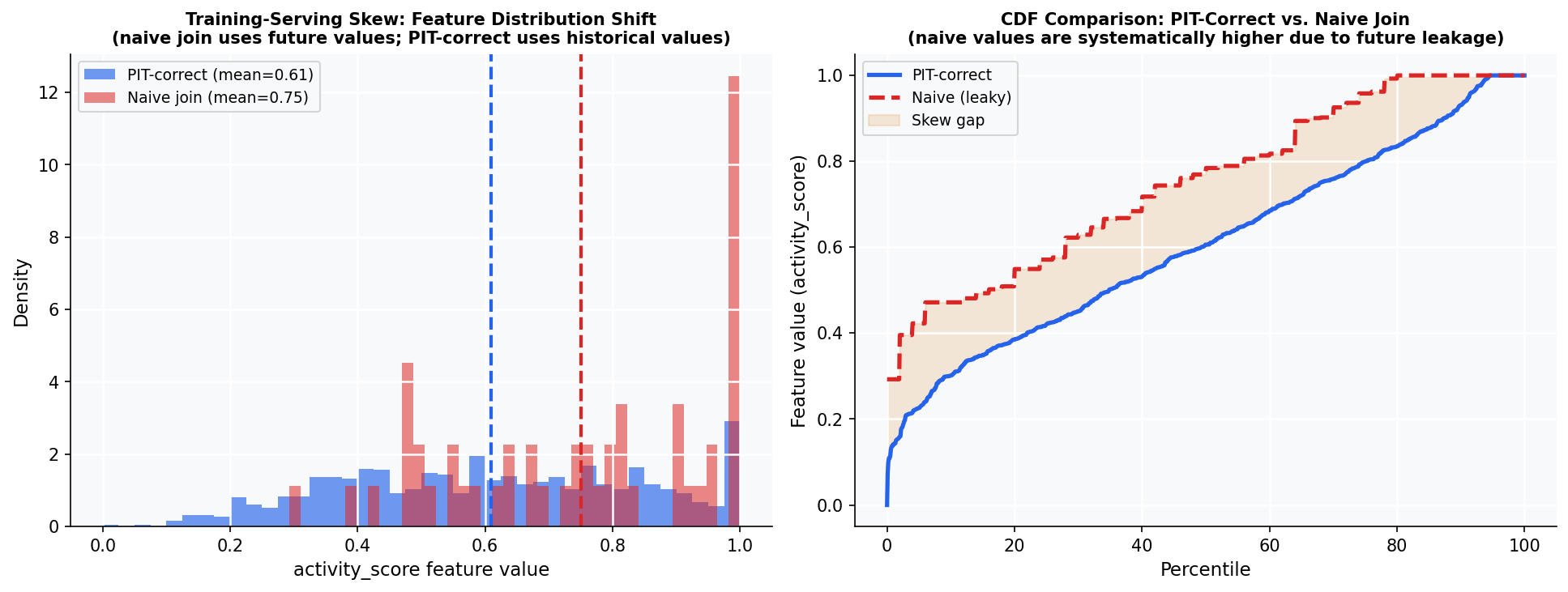 Figure 1: Feature value distribution and CDF for PIT-correct vs. naive joins on the same 1,000 events.
The histogram tells you the skew is structural, not noise: the blue PIT-correct distribution is roughly uniform across [0.2, 0.9], reflecting the underlying spread of activity levels per user. The red naive distribution is squeezed to the right, with a thick mode near 0.85 — these are users whose latest available activity_score was computed at the end of the 30-day window after the trend 0.01 * day had pushed every user’s score up. The CDF view sharpens this: the naive curve sits uniformly above the PIT curve, and the amber wedge between them has roughly constant vertical width, which means the bias is additive in feature value (≈+0.14 across all percentiles) rather than multiplicative. Additive bias is the worst kind for a threshold-based model, because the entire decision boundary moves by the same amount the features did.
The distortion visible in Figure 1 translates directly into the metric numbers below. The “classifier” here is intentionally trivial: a fixed threshold rule that predicts a click whenever the feature value exceeds 0.5, with ground-truth labels generated by drawing Uniform(0,1) < pit_value so the PIT-correct feature is by construction the calibrated probability the model is trying to recover. The point is to isolate the effect of feature skew alone, not to demonstrate a trained model.
| Statistic | PIT-correct join | Naive join | Delta |
|---|---|---|---|
Mean activity_score | 0.609 | 0.750 | +0.141 |
Std activity_score | 0.232 | 0.203 | -0.029 |
| Precision @ 0.5 threshold | 0.741 | 0.652 | -0.089 |
| Recall @ 0.5 threshold | 0.809 | 0.918 | +0.109 |
| F1 @ 0.5 threshold | 0.773 | 0.763 | -0.011 |
Two things are worth noticing. First, F1 barely moves — which is exactly why offline metrics fail to flag the bug. Second, the precision/recall asymmetry tells you what will hurt in production: a model trained with the naive join believes most users will click, so it fires too eagerly; precision drops because of the false positives, recall rises because the threshold is effectively shifted. When you redeploy with truthful (PIT-correct) serving-time features, the model’s calibration is wrong by exactly the +0.14 it learned to expect.
Methodology and data sources
The numbers in this article come from two places: a small reproducible simulation and well-documented public latency/freshness ranges for production storage backends. I want to be precise about what each figure rests on so a reader can change the assumptions and see how much the conclusions move.
Simulation (Figures 1 and 3). The simulation builds a synthetic dataset of 50 users, each with one activity_score value written to the offline store every 6 hours over 30 days (base_time = 2026-01-01), seeded with np.random.default_rng(42). Each user has a baseline activity drawn uniformly from [0.1, 0.9], plus a daily drift of 0.01 and Gaussian noise (std 0.05), clipped to [0, 1]. 1,000 training events are sampled at random (day, hour) pairs within the 30-day window. The click label for each event is generated by drawing Uniform(0,1) < pit_value, where pit_value is the PIT-correct feature at event time — so the label generation is the ground-truth signal the model is trying to recover. The skew table and Figure 1 then compare the PIT-correct join (only values with timestamp <= event_time) against the naive join (always latest available value). Figure 3 repeats the PIT join while sweeping max_staleness_hours ∈ {1, 2, 4, 6, 12, 24, 48, 168}. The threshold rule used in the metrics table is score > 0.5; all reported precision, recall, and F1 come from that rule applied to the joined feature value.
Storage latency and freshness ranges (Figure 2). The latency bars in Figure 2 are illustrative ranges based on publicly documented behaviour of each backend: Redis single-node sub-millisecond reads, DynamoDB single-digit-millisecond P99 in-region, Bigtable similar at scale, and Hive/Spark SQL in the tens-of-seconds-to-minutes regime for partitioned table scans. The staleness ranges on the right panel come from the published latency profiles of stream and micro-batch systems (Kafka + Flink sub-minute P50, micro-batch around 5 minutes by configuration, hourly and daily Airflow-style batches at their cadence). The point of the chart is the orders-of-magnitude gap between tiers, not the exact millisecond values; substitute your own backend’s numbers and the architectural decision will not change.
What is not in the simulation. The simulation does not model network failures, late-arriving stream events, multi-feature joins (which compound staleness across features), or the cost of regenerating training data after a backfill. The “Common failure modes” table and the “Production Considerations” section cover those qualitatively. The intent of the simulation is to make the core skew/coverage/quality tradeoffs concrete and reproducible, not to replace a full feature-store benchmark.
The Point-in-Time Correct Join
The fix is simple to describe: for each training event at time T, use only feature values that were available before T. This is called a point-in-time (PIT) correct join. The implementation also accepts a max_staleness_hours parameter — the maximum age of a feature value relative to the event time that is still considered usable; values older than this threshold are returned as NaN rather than silently used.
from __future__ import annotations
from dataclasses import dataclass, field
from datetime import datetime, timedelta
from typing import Any, Optional


@dataclass
class FeatureRecord:
    entity_id:    str
    feature_name: str
    value:        float
    timestamp:    datetime


@dataclass
class TrainingEvent:
    entity_id:  str
    event_time: datetime
    label:      int   # 1=click, 0=no-click


class OfflineStore:
    """Append-only, time-series storage of all feature values with timestamps."""

    def __init__(self):
        self._records: list[FeatureRecord] = []

    def write(self, rec: FeatureRecord) -> None:
        self._records.append(rec)

    def point_in_time_join(
        self,
        events: list[TrainingEvent],
        feature_names: list[str],
        max_staleness_hours: float = 24.0,
    ) -> list[dict]:
        results = []
        for ex in events:
            feat_vals: dict[str, Any] = {"entity_id": ex.entity_id, "label": ex.label}
            for fname in feature_names:
                # Only consider values BEFORE the event timestamp
                candidates = [
                    r for r in self._records
                    if r.entity_id == ex.entity_id
                    and r.feature_name == fname
                    and r.timestamp <= ex.event_time   # PIT constraint
                ]
                if candidates:
                    latest = max(candidates, key=lambda r: r.timestamp)
                    age_h = (ex.event_time - latest.timestamp).total_seconds() / 3600
                    if age_h <= max_staleness_hours:
                        feat_vals[fname] = latest.value
                    else:
                        feat_vals[fname] = float("nan")  # too stale
                else:
                    feat_vals[fname] = float("nan")  # no history
            results.append(feat_vals)
        return results

    def naive_join(
        self,
        events: list[TrainingEvent],
        feature_names: list[str],
    ) -> list[dict]:
        """Bug: uses latest available value regardless of event time."""
        results = []
        for ex in events:
            feat_vals: dict[str, Any] = {"entity_id": ex.entity_id, "label": ex.label}
            for fname in feature_names:
                # No PIT constraint — uses future values!
                candidates = [
                    r for r in self._records
                    if r.entity_id == ex.entity_id and r.feature_name == fname
                ]
                if candidates:
                    latest = max(candidates, key=lambda r: r.timestamp)
                    feat_vals[fname] = latest.value
                else:
                    feat_vals[fname] = float("nan")
            results.append(feat_vals)
        return results
The PIT join requires storing the full history of feature values — not just the current value — with timestamps. This is what the offline store provides.
The Dual-Store Architecture
PIT-correct joins require storing the full history of feature values with timestamps, which means the storage system itself must be designed with two distinct tiers — one optimised for historical queries and one for real-time lookup.
A feature store has two storage tiers:
Offline store (historical feature values):
- Append-only, time-series storage of all feature values with timestamps
- Supports PIT-correct joins for training data generation
- Examples: Hive tables, BigQuery, Delta Lake, Apache Iceberg partitioned by entity + time
- Query pattern: range scan over (entity_id, feature_name, timestamp)
- Latency: seconds to hours (batch access)
Online store (current feature values):
- Key-value store for low-latency feature lookup at serving time
- Stores only the latest value per (entity, feature)
- Examples: Redis, DynamoDB, Bigtable, Cassandra
- Query pattern: point lookup by entity_id
- Latency: < 10ms (P99)
class OnlineStore:
    """Key-value store for low-latency feature lookup."""

    def __init__(self):
        # key: (entity_id, feature_name) → (value, timestamp)
        self._store: dict[tuple[str, str], tuple[float, datetime]] = {}

    def write(self, rec: FeatureRecord) -> None:
        key = (rec.entity_id, rec.feature_name)
        existing = self._store.get(key)
        if existing is None or rec.timestamp > existing[1]:
            self._store[key] = (rec.value, rec.timestamp)

    def read(
        self,
        entity_id: str,
        feature_name: str,
        now: datetime,
        max_staleness_hours: float = 1.0,
    ) -> Optional[float]:
        key = (entity_id, feature_name)
        if key not in self._store:
            return None
        value, ts = self._store[key]
        age_hours = (now - ts).total_seconds() / 3600
        if age_hours > max_staleness_hours:
            return None   # stale feature → fallback or default
        return value

    def batch_read(
        self,
        entity_id: str,
        feature_names: list[str],
        now: datetime,
    ) -> dict[str, Optional[float]]:
        return {
            fname: self.read(entity_id, fname, now)
            for fname in feature_names
        }
The critical property: the feature computation logic is shared between the two stores. The same function that computes activity_score for offline batch processing also runs in the real-time serving pipeline. You write the transformation once; it materialises in both stores.
Feature Pipeline Architecture
The dual-store layout defines the destination for feature data; the pipeline architecture defines how feature values get there — and ensuring the two stores always reflect the same computation logic is where most real-world skew originates.
Features flow through the system via two pipelines that must stay consistent:
Batch pipeline (offline):
Raw logs → Spark/Beam → Feature computation → Offline store (Hive/Iceberg)
                                           → Online store snapshot (weekly refresh)
Stream pipeline (near-real-time):
Event stream (Kafka) → Flink/Spark Streaming → Feature computation
                                             → Online store (Redis, sub-minute)
                                             → Offline store (every 5 min append)
The key principle: the batch and stream pipelines implement the same transformation. For a windowed aggregate feature, the batch pipeline recomputes the full window from historical data, and the stream pipeline maintains a rolling state updated on each event. Both call into the same Python function, exported from a shared feature library — when the definition changes, both pipelines pick it up in the next release. Using a single canonical function in both pipelines eliminates implementation-level skew, a common source of bugs when teams maintain separate batch and streaming codebases.
The Consistency Challenge
Ensuring that offline and online feature values are consistent is harder than it sounds. Common failure modes:
Different implementations: The batch job is written in SQL and the streaming job is written in Python. Small differences in window boundary handling, timezone treatment, or NULL handling create systematic divergence.
Backfill gaps: When a new feature is launched, the offline store is backfilled from historical data. But the online store needs to be bootstrapped from a batch snapshot. If the backfill takes 2 days to complete and new events are streaming in, there is a window where the offline store has correct historical values but the online store has stale bootstrapped values.
Late-arriving events: Stream processors must decide when to close a time window. An event that arrives 30 minutes late might not be counted in the streaming window but would be counted in the batch recomputation. The offline store may show higher feature values than the online store for the same entity.
Latency and Freshness Across Storage Tiers
The dual-store design is justified by the latency gap between the workloads each tier serves; the staleness gap between the pipelines that feed them is what makes “fresh enough” a per-feature decision. Figure 2 shows both gaps side by side on a log scale.
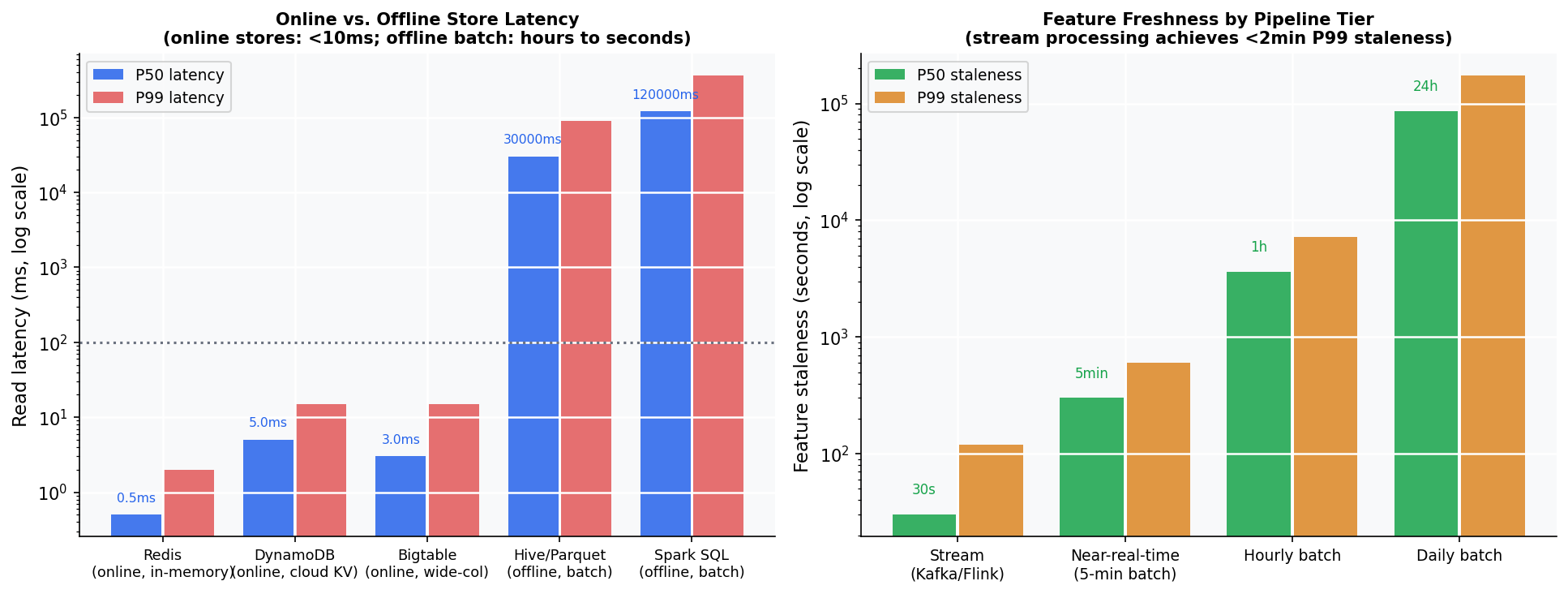 Figure 2: Read latency by storage backend (left) and feature staleness by pipeline tier (right). (Illustrative ranges from public docs.)
The left panel makes the architectural decision look obvious: in-memory and cloud key-value stores serve features in single-digit milliseconds at P99, well under the 100ms SLA budget that most synchronous inference paths can afford. Batch backends are four to six orders of magnitude slower — Hive at 30 seconds P50 is fine for training-set generation but unusable in a request path, and Spark SQL at two minutes is purely for offline aggregation. The right panel explains why the online store is not enough on its own: even with sub-10ms reads, the feature value behind that key is only as fresh as the pipeline that wrote it. Stream processing through Kafka and Flink can keep P99 staleness under two minutes; the 5-minute mini-batch tier doubles that; hourly and daily batches sit two and four orders of magnitude further out. Mixing tiers is therefore unavoidable: a fraud model wants the 30-second stream tier for session features but the daily batch tier for demographic features, and the online store is the place where both end up co-located behind a single point lookup.
Feature Freshness and Model Quality
Consistency between offline and online stores is a correctness requirement; the right freshness level for each feature is a separate decision that directly shapes which pipeline tier to use.
Not all features need the same freshness. Mixing feature tiers is common in production:
| Feature type | Example | Update frequency | Store tier |
|---|---|---|---|
| Real-time signals | Current session length | Per event | Stream → Online |
| Near-real-time | Last 1-hour click rate | 5-minute batch | Mini-batch → Online |
| Daily aggregates | 7-day engagement | Daily batch | Batch → Online snapshot |
| Quasi-static | User age, country | Weekly or on-change | Batch → Online |
The correct freshness requirement is determined by the feature’s temporal sensitivity: how much does the feature value change between the time a user’s session starts and when the model inference runs? A real-time session feature can change in seconds; a 7-day rolling aggregate changes by at most 1/7 per day.
Choosing a Staleness Threshold
Once you have a PIT-correct join, the next knob is the maximum age of feature values you accept. Too strict and most training events drop out for lack of a feature; too permissive and you train on values that no longer reflect the user’s state. Figure 3 sweeps the staleness threshold from 1 hour to 1 week against the same 1,000-event simulation, varying only max_staleness_hours in the PIT join.
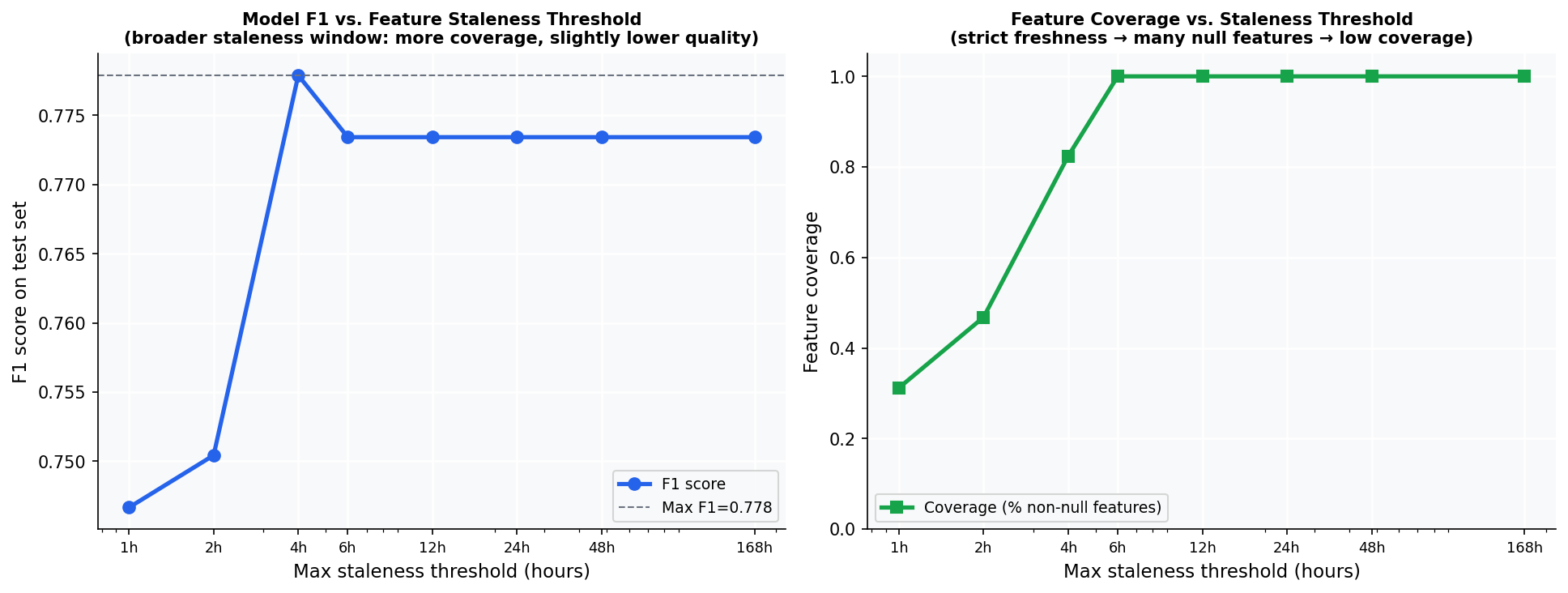 Figure 3: F1 (left) and feature coverage (right) as the maximum allowed feature staleness sweeps from 1 hour to 1 week.
Two things to read off the panels. First, the coverage curve on the right plateaus quickly: by the time you allow a 6-hour staleness window, nearly every event in this simulation has a usable historical feature, because the simulated feature is refreshed every 6 hours per user. The 1-hour threshold drops coverage sharply because most events fall in the gap between scheduled refreshes. Second, the F1 curve on the left is essentially flat once coverage stabilises — the simulated activity_score drifts by only 0.01 * day, so a 24-hour-old value carries almost the same information as a 1-hour-old value. Real features behave very differently depending on temporal sensitivity: a session-level feature loses most of its signal in minutes, while a 7-day rolling aggregate barely moves in a day. The practical rule is to pick the staleness threshold to match the feature’s update cadence (so coverage stabilises) and to validate empirically that F1 has plateaued, rather than picking a number out of a runbook. The chart shape is the diagnostic; the absolute hours are domain-specific.
Production Considerations
With freshness requirements defined, the remaining production challenges shift from individual feature correctness to operating features reliably across teams and over time.
Feature registry: In large organisations, dozens of teams compute features independently. Without a registry, duplicate features proliferate (team A computes user_7d_clicks; team B computes weekly_user_clicks; same computation, different names). A feature registry stores metadata: feature name, computation logic, owner, data sources, SLA, and monitoring thresholds. Feast and Tecton both provide registries; some organisations build internal ones.
Feature monitoring: Feature values drift as the underlying user behaviour changes. A feature that used to have mean 0.6 now has mean 0.3 — is this because the model should be retrained, or because there’s a pipeline bug? Production feature stores monitor:
- Distribution drift (KS test, PSI — Population Stability Index) compared to training baseline
- Null rate (unexpected increase in missing values)
- Freshness (age of the latest value in the online store)
- Volume (number of entities with recent values)
Backfilling new features: Launching a new feature requires:
- Implement the transformation
- Backfill historical values in the offline store (usually a one-time batch job)
- Bootstrap the online store from the backfill snapshot
- Start the real-time pipeline
- Regenerate training data with the new feature using PIT join
Step 5 is expensive — regenerating training data for a 90-day window on millions of users can take hours. Invest in fast backfill infrastructure early.
When You Don’t Need a Feature Store
Feature stores add significant engineering complexity. They are worth it when:
- You have multiple models sharing features (store computes once, shares)
- Your features require sub-minute freshness (stream processing is non-trivial)
- Training-serving skew is causing measurable performance degradation
- You have many teams producing features with inconsistent computation
They are not worth it when:
- You have a small number of models with simple, slowly-changing features
- Features are request-scoped (computed at inference time from request context)
- You are in a prototyping phase (feature store adds months to setup)
- Features don’t need historical PIT joins (e.g., features based only on the current request)
For most teams in the early stages of ML productionisation, a well-structured feature computation module with clear interfaces is sufficient. Invest in a feature store when you have demonstrated demand across multiple teams.
Summary
| Component | Role | Examples |
|---|---|---|
| Offline store | Historical time-series values; PIT joins | Hive, BigQuery, Iceberg |
| Online store | Current values; low-latency serving | Redis, DynamoDB, Bigtable |
| Transformation layer | Shared computation logic | Spark, Flink, dbt (data build tool — SQL-based transformation framework) |
| Feature registry | Metadata, discovery, governance | Feast, Tecton, internal |
| Monitoring | Distribution drift, freshness, nulls | Great Expectations (open-source data-quality library), custom |
Training-serving skew is not a modelling problem — it is a data engineering problem. The PIT join is the core primitive that prevents future leakage in training data. The dual-store architecture ensures that the same feature computation runs in both training and serving contexts. Feature stores operationalise these patterns at the scale of an organisation.
Incremental rollout: from ad-hoc features to a feature store
Most teams don’t start with a feature store. They start with feature code duplicated across training notebooks and inference services. The skew accumulates silently until a production regression surfaces it.
A practical migration path:
Phase 1 — shared feature library. Extract all feature computation into a Python library imported by both training and serving. This eliminates logical divergence even without a dedicated store. Cost: 1–2 engineer-weeks. Benefit: eliminates the most common skew class.
Phase 2 — offline store + PIT joins. Land feature time-series in a columnar store (BigQuery, Iceberg) and migrate training pipelines to use PIT joins. Cost: 2–4 weeks. Benefit: eliminates temporal leakage.
Phase 3 — online store. Add a Redis or DynamoDB online store and a write path that keeps it synchronized with the offline store. Cost: 4–8 weeks. Benefit: low-latency serving with feature reuse.
Phase 4 — registry and governance. Add a feature registry with metadata, ownership, and freshness SLAs. Cost: ongoing. Benefit: discoverability across teams, prevents redundant feature computation.
Most teams get 80% of the value by completing Phase 2. Phases 3–4 matter most when multiple models share features and when feature freshness directly impacts model quality (recommendation, fraud, pricing).
Common failure modes
The incremental migration path reduces risk, but several failure modes surface consistently across teams regardless of how carefully the rollout is staged.
| Failure mode | Root cause | Fix |
|---|---|---|
| Silent skew | Feature code diverged between training and serving | Shared library; integration test that compares outputs |
| Stale features | Online store write lag | Monitor max_age_seconds; add freshness alerts |
| Point-in-time leakage | Training joins on event time, not label time | Explicit PIT join with label timestamp |
| Schema drift | Upstream data change not propagated | Feature versioning; schema contracts on write path |
| Cold start latency | Online store not warmed | Pre-compute features for active entities at deploy time |
The most insidious failure is silent skew — the model continues to produce predictions, but those predictions are based on different feature values than training assumed. It degrades model quality without triggering any error. The antidote is an integration test that computes the same feature for the same entity through the training pipeline and the serving pipeline and asserts they match within floating-point tolerance. Run it on every deployment.
Key takeaways
- Point-in-time correctness is the most important property of a feature store. Violating it causes training data to contain future information, producing optimistic offline metrics that don’t hold in production.
- Offline and online stores serve different masters. Offline stores optimize for bulk reads and historical joins; online stores optimize for single-key lookups under 10ms. The transformation logic must be identical between them.
- A shared feature library eliminates the most common skew class without requiring a full feature store platform — it is the highest-value, lowest-cost first step.
- Freshness SLAs should be defined per feature, not per store. A user’s last purchase timestamp needs to be fresh within minutes for a pricing model; demographic features can tolerate hours.
- Monitoring is not optional. Distribution drift in input features is the most common cause of silent model degradation post-deployment. Track mean, variance, and null rate for every feature served to production and alert on deviations above two standard deviations from the training distribution.
- Start with a shared library, not a platform. Most teams don’t need Feast or Tecton on day one. A well-factored Python package with a clear interface between training and serving eliminates 80% of skew issues at a fraction of the operational cost. Add a dedicated store when you have multiple teams or multiple models sharing features at scale.
The architecture described here — shared transformation logic, PIT-correct training joins, dual offline/online stores, and drift monitoring — is the production-grade foundation for any ML system where model quality is business-critical. The investment pays back the first time it prevents a silent-skew regression from reaching your users.
A practical starting checklist:
- Extract all feature computation into a shared library — no divergent logic.
- Add a PIT join test: train on historical data, verify no future values are present.
- Add a feature freshness dashboard showing the age of each online store entry.
- Write one integration test that asserts training and serving produce identical feature values for the same entity and timestamp.