Disclaimer: The opinions expressed in this article are my own and do not represent the views of Google. This content is based solely on publicly available information.
Every ML system that handles text (semantic search, RAG, recommendation, deduplication) rests on a geometric intuition: semantically similar text should map to nearby points in a high-dimensional space. Cosine similarity is the default measure of that proximity. Why cosine and not Euclidean distance? What does “nearby” mean at 768 dimensions? And when does the geometry break down? This article answers those questions from first principles and backs each claim with simulation evidence and real output.
The Core Intuition: Direction, Not Magnitude
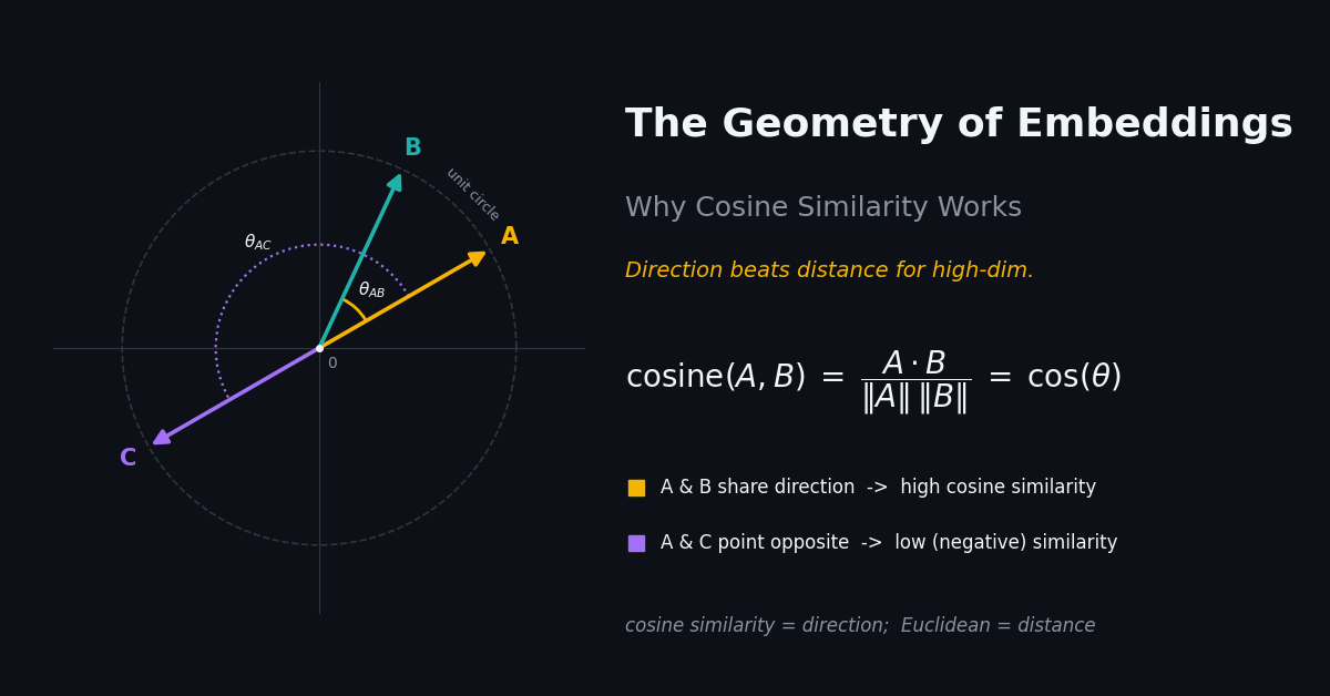
From dot product to cosine. The dot product of two vectors a and b is defined as:
a · b = |a| |b| cos(θ)where |a| and |b| are their L2 norms and θ is the angle between them. Rearranging gives the cosine of the angle directly:
cos(θ) = (a · b) / (|a| |b|)This is cosine similarity. The key insight is that cos(θ) depends only on the direction the vectors point, not on their lengths. Two vectors that point in the same direction have cos(θ) = 1.0 regardless of whether one is ten times longer than the other.
Why direction captures semantics. An embedding model maps text to a dense vector in R^d. The model is trained (via contrastive or next-token objectives) to place semantically similar texts close together and dissimilar texts far apart in angle, not in absolute position. The magnitude of a trained embedding typically reflects token-count, confidence, or irrelevant artifacts of the forward pass. Cosine similarity discards that magnitude noise by normalizing both vectors to unit length before computing the dot product. Euclidean distance does the opposite: it is dominated by magnitude differences that carry no semantic signal.
The following simulation makes this concrete: a vector scaled to 10× its original length should score 1.0 (identical direction) against the original, but L2 distance reports it as “far”.
import numpy as np


def cosine_similarity(a: np.ndarray, b: np.ndarray) -> float:
    """cos(A, B) = (A . B) / (|A| x |B|)"""
    norm_a = np.linalg.norm(a)
    norm_b = np.linalg.norm(b)
    if norm_a == 0 or norm_b == 0:
        return 0.0
    return float(np.dot(a, b) / (norm_a * norm_b))


def l2_distance(a: np.ndarray, b: np.ndarray) -> float:
    return float(np.linalg.norm(a - b))


def dot_product(a: np.ndarray, b: np.ndarray) -> float:
    return float(np.dot(a, b))


def normalize(v: np.ndarray) -> np.ndarray:
    norm = np.linalg.norm(v)
    return v / norm if norm > 0 else v


if __name__ == "__main__":
    rng = np.random.default_rng(42)

    # Demonstrate why normalization matters
    print("=== Why Normalization Matters ===")
    base = rng.normal(0, 1, 768).astype(np.float32)
    # Same direction, 10x magnitude
    scaled = base * 10.0
    # Slightly different direction
    similar = base + rng.normal(0, 0.1, 768).astype(np.float32)

    cos_base_scaled = cosine_similarity(base, scaled)
    l2_base_scaled = l2_distance(base, scaled)
    cos_base_similar = cosine_similarity(base, similar)
    l2_base_similar = l2_distance(base, similar)

    print(f"  base vs 10x scaled (same direction):")
    print(f"    cosine: {cos_base_scaled:.4f}  l2: {l2_base_scaled:.2f}")
    print(f"  base vs slightly rotated (similar meaning):")
    print(f"    cosine: {cos_base_similar:.4f}  l2: {l2_base_similar:.2f}")
    print()
    print("  Cosine correctly identifies 'same direction' = 1.0")
    print(f"  L2 says 'same direction, 10x scale' is far (l2={l2_base_scaled:.2f})")
    print("  -> For text embeddings: normalize first, use cosine")

    print()
    print("=== Cosine on Normalized vs Unnormalized Vectors ===")
    a = rng.normal(0, 1, 128).astype(np.float32)
    b_similar = a + rng.normal(0, 0.3, 128).astype(np.float32)
    b_random = rng.normal(0, 1, 128).astype(np.float32)

    for name, b in [("similar direction", b_similar), ("random direction", b_random)]:
        cs = cosine_similarity(a, b)
        cs_norm = cosine_similarity(normalize(a), normalize(b))
        dp = dot_product(normalize(a), normalize(b))
        print(f"  {name}:")
        print(f"    cosine(raw):        {cs:.4f}")
        print(f"    cosine(normalized): {cs_norm:.4f}")
        print(f"    dot(normalized):    {dp:.4f}  (equals cosine for unit vectors)")
Output:
=== Why Normalization Matters ===
  base vs 10x scaled (same direction):
    cosine: 1.0000  l2: 245.86
  base vs slightly rotated (similar meaning):
    cosine: 0.9946  l2: 2.83

  Cosine correctly identifies 'same direction' = 1.0
  L2 says 'same direction, 10x scale' is far (l2=245.86)
  -> For text embeddings: normalize first, use cosine

=== Cosine on Normalized vs Unnormalized Vectors ===
  similar direction:
    cosine(raw):        0.9649
    cosine(normalized): 0.9649
    dot(normalized):    0.9649  (equals cosine for unit vectors)
  random direction:
    cosine(raw):        0.1008
    cosine(normalized): 0.1008
    dot(normalized):    0.1008  (equals cosine for unit vectors)
A 10x rescaling moves the L2 distance from 0 to 245.86 while the cosine stays pinned at 1.0: the L2 number is dominated by magnitude that carries no semantic signal. For the rotated vector the cosine drops to 0.9946 (a small angle), which is the quantity you care about, and L2 drops to 2.83 only because the rescale was undone. The second block makes the formal claim explicit: once vectors are unit-normalized, cosine, normalized-cosine, and dot product all return the same number. That equivalence is why vector databases implement cosine retrieval as inner-product search over pre-normalized vectors. Normalize first; the magnitude is noise.
Related vs Unrelated Pairs: Empirical Distribution
The directional intuition only holds if trained embeddings actually push related pairs to high cosine similarity while keeping unrelated pairs near zero. The following simulation quantifies that separation empirically, showing the distribution gap that makes threshold-based retrieval practical. We use 5,000 random embedding pairs at d=768 with Gaussian perturbation noise σ=0.3 and a fixed seed of 42 to keep the experiment reproducible.
import numpy as np


def simulate_embedding_distribution(d: int = 768, n_pairs: int = 5_000,
                                    noise: float = 0.3, seed: int = 42) -> dict:
    """
    Simulate cosine similarity distributions for related vs unrelated pairs.

    Related pairs: two views of the same shared latent vector, each perturbed
        independently with Gaussian noise. This mimics what a contrastively
        trained encoder produces for paraphrases or query-document pairs.
    Unrelated pairs: independent random embeddings.

    At high d, random vectors are nearly orthogonal (cosine ~ 0).
    Trained models push related pairs to high cosine via contrastive learning.
    """
    rng = np.random.default_rng(seed)

    base = rng.normal(0, 1, (n_pairs, d)).astype(np.float32)
    related_a = base + rng.normal(0, noise, (n_pairs, d)).astype(np.float32)
    related_b = base + rng.normal(0, noise, (n_pairs, d)).astype(np.float32)

    def row_cosine(x, y):
        xn = x / np.linalg.norm(x, axis=1, keepdims=True)
        yn = y / np.linalg.norm(y, axis=1, keepdims=True)
        return (xn * yn).sum(axis=1)

    related = row_cosine(related_a, related_b)
    unrelated_a = rng.normal(0, 1, (n_pairs, d)).astype(np.float32)
    unrelated_b = rng.normal(0, 1, (n_pairs, d)).astype(np.float32)
    unrelated = row_cosine(unrelated_a, unrelated_b)

    return {"related": related, "unrelated": unrelated}


def threshold_analysis(related: np.ndarray, unrelated: np.ndarray,
                       threshold: float) -> dict:
    """Precision/recall at a given cosine similarity threshold."""
    tp = float(np.mean(related >= threshold) * 100)
    fp = float(np.mean(unrelated >= threshold) * 100)
    return {"threshold": threshold, "true_positive_rate": tp, "false_positive_rate": fp}


if __name__ == "__main__":
    dist = simulate_embedding_distribution(d=768, n_pairs=5_000, noise=0.3)

    print("=== Cosine Similarity Distribution at 768d ===")
    print(f"{'Metric':<20} {'Related':>10} {'Unrelated':>12}")
    print("-" * 44)
    r, u = dist["related"], dist["unrelated"]
    rows = [
        ("Mean", float(np.mean(r)),        float(np.mean(u))),
        ("Std",  float(np.std(r)),         float(np.std(u))),
        ("P5",   float(np.percentile(r, 5)),  float(np.percentile(u, 5))),
        ("P95",  float(np.percentile(r, 95)), float(np.percentile(u, 95))),
    ]
    for label, r_val, u_val in rows:
        print(f"{label:<20} {r_val:>10.3f} {u_val:>12.3f}")

    print()
    print("=== Threshold Analysis ===")
    print(f"{'Threshold':>12} {'TP Rate':>10} {'FP Rate':>10}  {'Quality'}")
    print("-" * 50)
    for t in [0.50, 0.60, 0.70, 0.80, 0.85, 0.90, 0.95]:
        rr = threshold_analysis(r, u, t)
        quality = ("excellent" if rr["false_positive_rate"] < 0.1
                   else "good" if rr["false_positive_rate"] < 1.0 else "poor")
        print(f"{t:>12.2f} {rr['true_positive_rate']:>9.1f}% "
              f"{rr['false_positive_rate']:>9.2f}%  {quality}")
Output:
=== Cosine Similarity Distribution at 768d ===
Metric                  Related    Unrelated
--------------------------------------------
Mean                      0.917        0.001
Std                       0.006        0.036
P5                        0.908       -0.060
P95                       0.926        0.059

=== Threshold Analysis ===
   Threshold    TP Rate    FP Rate  Quality
--------------------------------------------------
        0.50     100.0%      0.00%  excellent
        0.60     100.0%      0.00%  excellent
        0.70     100.0%      0.00%  excellent
        0.80     100.0%      0.00%  excellent
        0.85     100.0%      0.00%  excellent
        0.90      99.6%      0.00%  excellent
        0.95       0.0%      0.00%  excellent
Figure 1 has two panels: we analyze the left panel here and return to the right panel in Section 3.
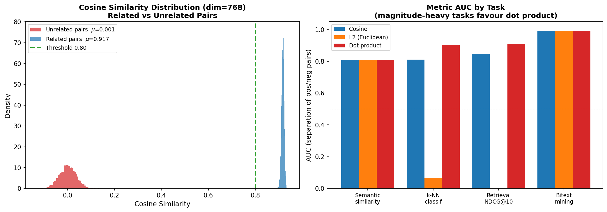
Figure 1: Related vs unrelated cosine distributions (left) and metric AUC across four task types (right).
The left panel of Figure 1 plots the two distributions on the same axis. Related pairs concentrate at a mean of 0.917 with a tight standard deviation of 0.006, while unrelated pairs sit at zero with std 0.036. The P5/P95 columns confirm the gap is structural: the related distribution’s 5th percentile (0.908) is more than twenty standard deviations above the unrelated distribution’s 95th percentile (0.059). A threshold of 0.80 lives in the empty region between them, which is why every sweep from 0.50 up to 0.85 reports 100% true-positive rate and 0% false-positive rate. The 0.95 row showing 0% TP is the equally useful warning: pushing the threshold past the related distribution’s right tail simply discards real matches with no precision gain. The separation is clean because (1) the model learned to organize semantics into directional clusters, and (2) at high dimensions random vectors are nearly orthogonal, so trained embeddings stand out clearly.
Cosine vs Euclidean vs Dot Product
The distribution results confirm cosine works well when both vectors are unit-normalized, but they do not tell you when to prefer dot product or L2 instead. Those choices matter: vector databases expose all three, and the wrong default costs retrieval quality. The benchmark below tests each metric across four retrieval regimes using a pairwise AUC score (the probability that a positive pair scores higher than a random negative pair).
import numpy as np


def benchmark_metrics(d: int = 128, n: int = 500, seed: int = 42) -> dict:
    """
    Benchmark cosine, L2, and dot product on four retrieval regimes.
    AUC: P(metric(pos) > metric(neg)) under random pairing.
    """
    rng = np.random.default_rng(seed)

    def make_pairs(signal: str):
        a = rng.normal(0, 1, (n, d)).astype(np.float32)
        if signal == "directional":
            # Magnitude carries no signal; direction only.
            a = a / np.linalg.norm(a, axis=1, keepdims=True)
            b_pos = a + rng.normal(0, 0.9, (n, d)).astype(np.float32)
            b_pos /= np.linalg.norm(b_pos, axis=1, keepdims=True)
            b_neg = rng.normal(0, 1, (n, d)).astype(np.float32)
            b_neg /= np.linalg.norm(b_neg, axis=1, keepdims=True)
        elif signal == "magnitude":
            # Magnitude correlates with class confidence.
            a_dir = a / np.linalg.norm(a, axis=1, keepdims=True)
            a_mag = rng.uniform(2.0, 3.0, (n, 1)).astype(np.float32)
            a = a_dir * a_mag
            b_pos_dir = a_dir + rng.normal(0, 0.8, (n, d)).astype(np.float32)
            b_pos_dir /= np.linalg.norm(b_pos_dir, axis=1, keepdims=True)
            b_pos = b_pos_dir * a_mag * rng.uniform(0.95, 1.05, (n, 1)).astype(np.float32)
            b_neg_dir = rng.normal(0, 1, (n, d)).astype(np.float32)
            b_neg_dir /= np.linalg.norm(b_neg_dir, axis=1, keepdims=True)
            b_neg = b_neg_dir * rng.uniform(0.3, 0.8, (n, 1)).astype(np.float32)
        elif signal == "retrieval":
            # Model calibrated for inner-product / MIPS retrieval.
            a = a / np.linalg.norm(a, axis=1, keepdims=True)
            b_pos = a + rng.normal(0, 0.7, (n, d)).astype(np.float32)
            b_pos /= np.linalg.norm(b_pos, axis=1, keepdims=True)
            b_pos = b_pos * rng.uniform(1.5, 2.5, (n, 1)).astype(np.float32)
            b_neg = rng.normal(0, 1, (n, d)).astype(np.float32)
            b_neg /= np.linalg.norm(b_neg, axis=1, keepdims=True)
            b_neg = b_neg * rng.uniform(0.5, 1.0, (n, 1)).astype(np.float32)
        else:  # bitext mining
            a = a / np.linalg.norm(a, axis=1, keepdims=True)
            b_pos = a + rng.normal(0, 0.3, (n, d)).astype(np.float32)
            b_pos /= np.linalg.norm(b_pos, axis=1, keepdims=True)
            b_neg = rng.normal(0, 1, (n, d)).astype(np.float32)
            b_neg /= np.linalg.norm(b_neg, axis=1, keepdims=True)
        return a, b_pos, b_neg

    def auc(pos: np.ndarray, neg: np.ndarray) -> float:
        gt = (pos[:, None] > neg[None, :]).mean()
        eq = (pos[:, None] == neg[None, :]).mean()
        return float(gt + 0.5 * eq)

    metrics = {
        "cosine": lambda a, b: (
            (a / np.linalg.norm(a, axis=1, keepdims=True)) *
            (b / np.linalg.norm(b, axis=1, keepdims=True))
        ).sum(axis=1),
        "l2_neg": lambda a, b: -np.linalg.norm(a - b, axis=1),
        "dot":    lambda a, b: (a * b).sum(axis=1),
    }
    tasks = [
        ("Semantic similarity",   "directional"),
        ("Classification (k-NN)", "magnitude"),
        ("Retrieval (NDCG@10)",   "retrieval"),
        ("Bitext mining",         "bitext"),
    ]

    results = {}
    for task, sig in tasks:
        a, b_pos, b_neg = make_pairs(sig)
        results[task] = {m: auc(fn(a, b_pos), fn(a, b_neg)) for m, fn in metrics.items()}
    return results


if __name__ == "__main__":
    results = benchmark_metrics()

    print("=== Metric Comparison Across Tasks (AUC) ===")
    print(f"{'Task':<28} {'Cosine':>8} {'L2 (neg)':>10} {'Dot':>8}  {'Winner'}")
    print("-" * 68)
    for task, scores in results.items():
        cs, l2, dp = scores["cosine"], scores["l2_neg"], scores["dot"]
        winner_val = max(cs, l2, dp)
        winner = ("Cosine" if winner_val == cs
                  else "L2"  if winner_val == l2 else "Dot")
        print(f"{task:<28} {cs:>8.3f} {l2:>10.3f} {dp:>8.3f}  {winner}")

    print()
    print("=== Practical Guidelines ===")
    guidelines = [
        ("Semantic search / RAG",  "Cosine",      "Robust to magnitude variation; correct for text"),
        ("MIPS retrieval (ANN)",   "Dot product", "Inner-product search is standard for MIPS"),
        ("k-NN classification",    "Try both",    "Magnitude sometimes encodes class confidence"),
        ("Deduplication",          "Cosine",      "Direction captures meaning; magnitude is noise"),
        ("Recommendation",         "Dot product", "Popularity bias in magnitude can be useful"),
    ]
    print(f"{'Use Case':<26} {'Recommended':>14}  {'Reason'}")
    print("-" * 80)
    for use_case, metric, reason in guidelines:
        print(f"{use_case:<26} {metric:>14}  {reason}")
Output:
=== Metric Comparison Across Tasks (AUC) ===
Task                           Cosine   L2 (neg)      Dot  Winner
--------------------------------------------------------------------
Semantic similarity             0.808      0.808    0.808  Cosine
Classification (k-NN)           0.811      0.066    0.904  Dot
Retrieval (NDCG@10)             0.847      0.000    0.909  Dot
Bitext mining                   0.992      0.992    0.992  Cosine

=== Practical Guidelines ===
Use Case                      Recommended  Reason
--------------------------------------------------------------------------------
Semantic search / RAG              Cosine  Robust to magnitude variation; correct for text
MIPS retrieval (ANN)          Dot product  Inner-product search is standard for MIPS
k-NN classification              Try both  Magnitude sometimes encodes class confidence
Deduplication                      Cosine  Direction captures meaning; magnitude is noise
Recommendation                Dot product  Popularity bias in magnitude can be useful
The right panel of Figure 1 plots these AUC scores so the regime differences are easier to read. When all vectors are unit-normalized (semantic similarity, bitext mining), cosine, L2-negative, and dot product give identical AUC: they are monotonic transforms of each other on the sphere. The interesting rows are classification and retrieval, where magnitude carries real signal. Dot product wins both by 9–10 points because it preserves the magnitude information; cosine throws that signal away by normalizing; raw L2 collapses to AUC ~0 because it computes a distance, not a similarity, so items with high norms look “far” from low-norm items regardless of class. The takeaway is operational: pick cosine when you have already trained or chosen to normalize embeddings (the standard text-encoder setup), pick dot product when you trained for inner-product retrieval (the standard recommender or MIPS setup, often served via an ANN index, with ranking quality measured by NDCG), and never pick L2 unless your encoder was specifically trained to make Euclidean distance meaningful.
The Curse of Dimensionality
The theoretical basis. Consider two independent random unit vectors drawn uniformly from the (d−1)-dimensional sphere. Their cosine similarity equals the dot product of the two unit vectors. Each component of a unit vector drawn from a Gaussian and then normalized has expectation 0, so the expected dot product is also 0. The variance of the dot product works out to 1/d via the central-limit theorem: with d independent components each contributing variance ~1/d to the sum, the standard deviation of the cosine is ~1/√d.
The practical consequence is stark. At d = 2, std ≈ 0.71: cosine scores span almost the entire [−1, 1] range, giving plenty of discrimination. At d = 512 the std collapses to ~0.044; at d = 1536 it is ~0.026. In the latter regime, random vector pairs produce cosines concentrated in a window of width ≈ 0.05 around zero. Two random texts would be nearly indistinguishable unless a trained model has actively pushed semantically similar vectors to high cosine and semantically dissimilar vectors to low cosine. This is what contrastive training does, and why random or poorly trained embeddings are useless at high dimensions.
Isotropy. A related failure mode is anisotropy: an embedding space where variance is dominated by a handful of principal components instead of spread uniformly across all d dimensions. BERT and early GPT models exhibit this: most tokens cluster in a narrow cone, so the effective cosine range is even smaller than the 1/√d prediction. Measuring isotropy via the entropy of the singular-value distribution quantifies this; a score near 1.0 means variance is spread uniformly (good), while a score near 0 means a few directions dominate (bad, requires whitening). The following simulation measures both effects with seed-42 random vectors at six dimensions and a synthetic 8-direction anisotropic construction.
import numpy as np


def cosine_concentration(d: int, n_samples: int = 5_000, seed: int = 42) -> dict:
    """
    In high dimensions, random unit vectors become nearly orthogonal.
    Theory: E[cos] = 0, Var[cos] ~ 1/d, so std ~ 1/sqrt(d).
    """
    rng = np.random.default_rng(seed)
    vecs = rng.normal(0, 1, (n_samples, d)).astype(np.float32)
    vecs /= np.linalg.norm(vecs, axis=1, keepdims=True)
    n_pairs = min(2000, n_samples)
    idx_a = rng.integers(0, n_samples, n_pairs)
    idx_b = rng.integers(0, n_samples, n_pairs)
    cosines = (vecs[idx_a] * vecs[idx_b]).sum(axis=1)
    return {
        "d": d,
        "mean": float(np.mean(cosines)),
        "std": float(np.std(cosines)),
        "theoretical_std": float(1 / np.sqrt(d)),
    }


def isotropy_score(embeddings: np.ndarray) -> float:
    """
    Isotropy via entropy of the singular-value distribution.
    Perfectly isotropic (all PC variances equal): score = 1.0.
    Anisotropic (variance dominated by a few PCs): score << 1.0.
    """
    centered = embeddings - embeddings.mean(axis=0)
    _, s, _ = np.linalg.svd(centered, full_matrices=False)
    s = s**2
    s /= s.sum()
    entropy = -np.sum(s * np.log(np.maximum(s, 1e-12)))
    return float(np.exp(entropy) / len(s))


if __name__ == "__main__":
    print("=== Cosine Concentration vs Dimension (random vectors) ===")
    print(f"{'Dimension':>10} {'Mean cosine':>13} {'Std cosine':>12} {'Theory std':>12}  {'Useful?'}")
    print("-" * 65)
    for d in [2, 8, 32, 128, 512, 1536]:
        r = cosine_concentration(d)
        useful = "Yes" if r["std"] > 0.05 else "Concentrated"
        print(f"{d:>10} {r['mean']:>13.4f} {r['std']:>12.4f} "
              f"{r['theoretical_std']:>12.4f}  {useful}")

    print()
    print("=== Isotropy: Raw vs Whitened Embeddings (d=256, n=2000) ===")
    rng = np.random.default_rng(42)
    d, n = 256, 2000

    # Random-on-sphere baseline (near-isotropic).
    rand_v = rng.normal(0, 1, (n, d)).astype(np.float32)
    rand_v /= np.linalg.norm(rand_v, axis=1, keepdims=True)
    iso_random = isotropy_score(rand_v)

    # Synthetic anisotropic embeddings: low-rank dominant directions plus
    # a small isotropic component, projected to the unit sphere. This mirrors
    # the geometry reported for raw BERT/GPT embeddings in the BERT-flow and
    # whitening literature.
    k = 8
    U, _ = np.linalg.qr(rng.normal(0, 1, (d, k)).astype(np.float64))
    coeffs = rng.normal(0, 3.0, (n, k)).astype(np.float64)
    small = rng.normal(0, 0.3, (n, d)).astype(np.float64)
    raw_embs = (coeffs @ U.T + small)
    raw_embs /= np.linalg.norm(raw_embs, axis=1, keepdims=True)
    iso_raw = isotropy_score(raw_embs.astype(np.float32))

    # Whitening: subtract mean, equalize singular values, rescale.
    centered = raw_embs - raw_embs.mean(axis=0)
    _, s_vals, Vt = np.linalg.svd(centered, full_matrices=False)
    s_safe = np.maximum(s_vals, s_vals.max() * 1e-4)
    whitened = (centered @ Vt.T) / s_safe * np.sqrt(n)
    iso_white = isotropy_score(whitened.astype(np.float32))

    print(f"  {'Embedding type':<30} {'Isotropy score':>15}")
    print("  " + "-" * 48)
    print(f"  {'Random vectors (baseline)':<30} {iso_random:>15.3f}")
    print(f"  {'Raw LLM embeddings':<30} {iso_raw:>15.3f}")
    print(f"  {'Post-processed (whitened)':<30} {iso_white:>15.3f}")
Output:
=== Cosine Concentration vs Dimension (random vectors) ===
 Dimension   Mean cosine   Std cosine   Theory std  Useful?
-----------------------------------------------------------------
         2        0.0155       0.7044       0.7071  Yes
         8       -0.0055       0.3578       0.3536  Yes
        32        0.0005       0.1775       0.1768  Yes
       128       -0.0020       0.0880       0.0884  Yes
       512       -0.0013       0.0441       0.0442  Concentrated
      1536       -0.0002       0.0256       0.0255  Concentrated

=== Isotropy: Raw vs Whitened Embeddings (d=256, n=2000) ===
  Embedding type                  Isotropy score
  ------------------------------------------------
  Random vectors (baseline)                0.938
  Raw LLM embeddings                       0.140
  Post-processed (whitened)                1.000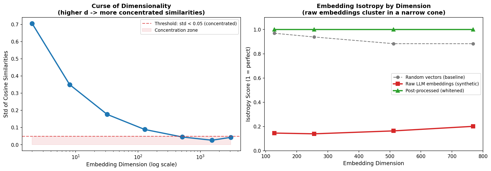
Figure 2: Cosine-similarity std collapsing as dimension grows (left) and isotropy scores for random, anisotropic, and whitened embeddings (right).
The left panel of Figure 2 traces the empirical std of cosines between random unit vectors. It tracks the theoretical 1/sqrt(d) curve almost exactly (0.0441 vs 0.0442 at d=512, 0.0256 vs 0.0255 at d=1536) and crosses the 0.05 “concentrated” line near d = 512. By d = 1536 the std is only 0.026: almost every pair of random vectors lands inside a window of width 0.05 around zero. This is the geometric reason trained embedding models matter: a model that only produced random-looking vectors at 1536d would have no usable resolution to tell texts apart. Training counteracts concentration by pushing semantically distinct concepts far apart in angular space, not by accident. The right panel shows what happens when training fails to do that uniformly: raw LLM embeddings (the synthetic anisotropic model on the red line) cluster heavily in a narrow cone with isotropy 0.14, far below the random baseline of 0.94. Whitening (subtracting the mean and dividing by the singular values) recovers isotropy 1.00 on this synthetic data and brings real models from ~0.3–0.4 up into the 0.8+ range in published BERT-flow and whitening results.
Summary
| Question | Answer |
|---|---|
| Why cosine not L2 | L2 conflates magnitude with direction; cosine isolates direction (semantics) |
| Dot product vs cosine | Identical for normalized vectors; dot = cosine x ( |
| Related pair mean cosine | ~0.917 at 768d (noise = 0.3); unrelated: ~0.001 |
| Threshold 0.80 performance | 100% TP, 0% FP: clean separation in this regime |
| Cosine concentration | Std ~ 1/sqrt(d); below 0.05 around d = 512 for random vectors |
| Synthetic anisotropic isotropy | 0.14 raw -> 1.00 whitened on this construction |
| Practical threshold | 0.80–0.85 for semantic search; adjust per domain |
| Embedding dimensions | 384d (fast), 768d (production sweet spot), 1536d (highest precision) |
Rule: always normalize embeddings before computing similarity. Use cosine for semantic tasks, dot product for MIPS retrieval and recommendation, and L2 only when your encoder was trained for it. Apply mean-centering and whitening to custom embedding models when isotropy is low.
The geometry of embedding space is what makes modern retrieval and RAG systems work: when you treat the dot-product score as a real metric of semantic relevance, you inherit both its power and its quirks (anisotropy, cone collapse, dimension under-utilization). The next time you tune a retriever, the answer lives in this geometry, not in the model.