
Disclaimer: The opinions expressed in this article are my own and do not represent the views of Google. This content is based solely on publicly available information.
TL;DR of Parts 1-3. Embeddings (Part 1) turn words into dense vectors. RNNs and LSTMs (Part 2) read those vectors in order but suffer from vanishing gradients and offer no parallelism. Scaled dot-product attention (Part 3) fixes both by letting every position read directly from every other position in one parallel matrix multiplication — but it has no notion of word order and uses only a single attention pattern. We fix both gaps in this part. See Part 3 for the mechanism we now extend.
Series navigation
| Part | Topic |
|---|---|
| 1 | Introduction & Word Embeddings |
| 2 | From RNNs to LSTMs |
| 3 | The Attention Mechanism |
| 4 (this article) | Multi-Head Attention & Positional Encoding |
| 5 | The Transformer Encoder |
| 6 | The Decoder & Full Transformer |
| 7 | Pre-trained Models & Tokenization |
| 8 | Supervised Fine-Tuning |
| 9 | LoRA & QLoRA |
| 10 | DPO Alignment |
In Part 3, we built scaled dot-product attention from scratch and confirmed that every position can read from every other position in one parallel matrix multiplication. That single-head mechanism has two gaps: it uses only one attention pattern, and it has no sense of where tokens sit in the sequence. This part patches both gaps, and by the end you will have assembled the complete attention block that appears verbatim inside every modern Transformer.
Recap from Part 3: scaled dot-product attention computes Q (queries), K (keys), V (values) from input embeddings, then mixes V via softmax(Q·K^T / √d_k). Multi-head attention runs this in parallel across h sub-spaces of dimension d_k = d_model / h.
In this part we cover the two upgrades that take us from “raw self-attention” to “the attention block actually used inside every Transformer”:
- Multi-Head Attention — run attention in parallel across several smaller subspaces, each free to learn a different kind of relation.
- Positional Encoding — inject explicit position information into the embeddings so the model can distinguish word order.
Why one head is not enough
Single-head attention is a solid foundation, but intuition says that language is too rich for one attention pattern to capture everything at once. This section makes that intuition concrete before we implement the multi-head extension.
A single attention head learns one matrix of attention weights — one kind of relationship between tokens. But a sentence carries many simultaneous relations:
- subject ↔ verb agreement
- pronoun ↔ antecedent coreference
- adjective ↔ noun modification
- punctuation ↔ clause boundaries
Forcing one attention pattern to capture all of these is like asking one person to listen to four conversations at once and accurately summarise each.
Multi-head attention splits the model dimension d across h independent heads. Each head gets d_k = d/h dimensions, computes its own Q, K, V (Q, K, V — query, key, value projections of the input, each shaped (seq_len, d_model/h) per head.), runs its own scaled dot-product attention, and produces its own output. Then we concatenate all the per-head outputs back to the full d-dimensional space and pass them through one more linear projection W^O.
flowchart LR
    Input["Input<br/>(seq, d=128)"] --> H1["Head 1<br/>d_k=32"]
    Input --> H2["Head 2<br/>d_k=32"]
    Input --> H3["Head 3<br/>d_k=32"]
    Input --> H4["Head 4<br/>d_k=32"]
    H1 --> Concat["Concat<br/>(seq, d=128)"]
    H2 --> Concat
    H3 --> Concat
    H4 --> Concat
    Concat --> Linear["Linear W^O"]
    Linear --> Output["Output<br/>(seq, d=128)"]
Figure 1: Multi-head attention with 4 parallel heads over a 128-dim model.
The diagram above traces the full path. Each head operates in its own 32-dim subspace (d_k = 128/4 = 32), runs scaled dot-product attention independently, and produces a 32-dim output per position. Concatenating the four head outputs returns us to a 128-dim tensor, which the final linear projection W^O mixes one last time to give the block’s output. Because every head shrinks its working dimension by exactly the factor 1/h, the total compute matches a single head operating over the full 128 dims — multi-head is a redistribution of capacity, not an addition. We are not making the model bigger; we are giving it more representational flexibility for the same parameter budget.
PyTorch’s built-in and a from-scratch version
Having established why multiple heads help, we can now implement them. This section shows both the one-liner that PyTorch ships out of the box and the from-scratch version that makes the reshape-and-split operation transparent — both produce identical outputs.
In PyTorch, multi-head attention is one line:
import torch
import torch.nn as nn

d_model, num_heads = 128, 4
mha = nn.MultiheadAttention(embed_dim=d_model, num_heads=num_heads, batch_first=True)

# Example forward pass
x      = torch.randn(2, 10, d_model)    # (batch=2, seq=10, d=128)
out, w = mha(x, x, x)                  # self-attention: q=k=v=x
print(f"Output shape  : {out.shape}")   # (2, 10, 128)
print(f"Weight shape  : {w.shape}")     # (2, 10, 10)
Output:
Output shape  : torch.Size([2, 10, 128])
Weight shape  : torch.Size([2, 10, 10])
If you prefer to see the mechanism explicitly, here is the from-scratch version:
import torch
import torch.nn as nn
import torch.nn.functional as F

class MultiHeadAttention(nn.Module):
    def __init__(self, d_model, num_heads):
        super().__init__()
        assert d_model % num_heads == 0
        self.h   = num_heads
        self.d_k = d_model // num_heads
        self.Wq  = nn.Linear(d_model, d_model)
        self.Wk  = nn.Linear(d_model, d_model)
        self.Wv  = nn.Linear(d_model, d_model)
        self.Wo  = nn.Linear(d_model, d_model)

    def forward(self, x):
        B, L, _ = x.shape
        # Project and split into (B, num_heads, L, d_k)
        Q = self.Wq(x).view(B, L, self.h, self.d_k).transpose(1, 2)
        K = self.Wk(x).view(B, L, self.h, self.d_k).transpose(1, 2)
        V = self.Wv(x).view(B, L, self.h, self.d_k).transpose(1, 2)

        scores  = (Q @ K.transpose(-2, -1)) / (self.d_k ** 0.5)  # (B, h, L, L)
        weights = F.softmax(scores, dim=-1)
        out     = weights @ V                                       # (B, h, L, d_k)

        # Recombine heads: (B, h, L, d_k) → (B, L, d_model)
        out = out.transpose(1, 2).contiguous().view(B, L, self.h * self.d_k)
        return self.Wo(out)

mha  = MultiHeadAttention(d_model=128, num_heads=4)
x    = torch.randn(2, 10, 128)
out  = mha(x)
print(f"Output shape : {out.shape}")      # (2, 10, 128)
n_params = sum(p.numel() for p in mha.parameters())
print(f"Parameters   : {n_params:,}")    # 66,048
Output:
Output shape : torch.Size([2, 10, 128])
Parameters   : 66,048
The single line Q.view(B, L, self.h, self.d_k).transpose(1, 2) is what splits the model into heads. The transpose rearranges from (B, L, h, d_k) to (B, h, L, d_k) so that each head’s attention matrix (L, L) can be computed with a single batched matmul over the h dimension.
What each head attends to
The from-scratch code shows the mechanics, but it does not tell us what patterns the heads actually learn on real text. This section summarises what empirical studies have found — giving you a mental vocabulary for interpreting multi-head attention in trained models.
With randomly initialized weights, the heads have no interpretable structure. After training on real text, empirical studies (Voita et al., 2019; Clark et al., 2019) show distinct roles emerge:
From Clark et al., 2019 (BERT-specific):
- Some heads act as delimiter aggregators, routing everything through
[SEP]tokens
From Voita et al., 2019 (encoder-decoder NMT):
- Some heads learn to attend to the immediately adjacent token (position-sensitive)
- Some heads attend to the subject of the verb even when the verb is far from the subject
- Some heads track coreference (pronoun → antecedent)
The number of heads h is a hyperparameter. GPT-2 (117M parameters) uses h=12 with d_k=64. GPT-3 (175B parameters) uses h=96 with d_k=128. The relationship d_k = d_model / h keeps the parameter count fixed regardless of how many heads you use.
The position problem
Multi-head attention solves the single-perspective limitation, but it inherits another flaw from its single-head parent: it is completely blind to the order of tokens. This section demonstrates that failure mode with a real measurement before showing the fix.
Self-attention is permutation-equivariant — shuffle the input order and the output gets shuffled in exactly the same way. A model that cannot distinguish “the dog chased the cat” from “the cat chased the dog” is useless for language.
Let us verify this failure mode:
# Reuses MultiHeadAttention (and positional_encoding) defined earlier; assumes top-to-bottom execution.
import torch

torch.manual_seed(0)
mha = MultiHeadAttention(d_model=128, num_heads=4)

x_original = torch.randn(1, 4, 128)   # tokens 0,1,2,3
x_shuffled = x_original[:, [2,0,3,1]] # tokens 2,0,3,1

out_orig    = mha(x_original)
out_shuffled = mha(x_shuffled)

# The shuffled output should be the shuffled version of the original
out_orig_reordered = out_orig[:, [2,0,3,1]]
diff = (out_shuffled - out_orig_reordered).abs().max()
print(f"Max difference (should be ~0): {diff.item():.2e}")
Output:
Max difference (should be ~0): 1.19e-07Confirmed: attention is indeed permutation-equivariant. If we shuffle the inputs, the outputs are shuffled in exactly the same way. The model has no notion of position.
Sine/cosine positional encoding
The position problem has a surprisingly clean solution: add a fixed mathematical signal to each token’s embedding before attention runs. Intuitively, each token’s vector gets a unique “fingerprint” that encodes its position, and because the signal is additive, attention layers can learn to read it without any change to their architecture. The formulas below make that fingerprint precise.
The trick the original Transformer paper introduced is beautifully simple: add a fixed position-dependent signal to every token’s embedding before any attention happens. The position signal must satisfy two properties:
- Different positions must get distinguishably different signals.
- The signal must generalise to position values the model has not seen during training (positions longer than any training sequence).
The choice they made was a sum of sine and cosine waves at geometrically spaced frequencies:
$$PE_{(pos,,2i)} = \sin!\left(\frac{pos}{10000^{2i/d_{model}}}\right)$$
$$PE_{(pos,,2i+1)} = \cos!\left(\frac{pos}{10000^{2i/d_{model}}}\right)$$
For each position pos and each pair of dimensions (2i, 2i+1), we get one sine value and one cosine value at a position-and-dimension-dependent frequency. The early dimensions oscillate quickly with position (they encode where roughly within a few-token window); the later dimensions oscillate slowly (they encode where across hundreds of positions). Together, every position gets a unique combination — its own “fingerprint” — that the model can learn to read.
The whole thing has zero trainable parameters. It is computed once, cached, and added.
Computing the PE matrix in PyTorch
The formulas translate into about ten lines of PyTorch and produce a tensor that we can immediately plot. The code below generates the matrix and prints a few rows so you can verify the wave-like structure numerically before we visualise it.
import torch

def positional_encoding(max_len: int, d_model: int) -> torch.Tensor:
    pos    = torch.arange(max_len).unsqueeze(1).float()           # (max_len, 1)
    i      = torch.arange(d_model // 2).unsqueeze(0).float()     # (1, d_model/2)
    angles = pos / (10000 ** (2 * i / d_model))                  # (max_len, d_model/2)
    pe     = torch.zeros(max_len, d_model)
    pe[:, 0::2] = torch.sin(angles)
    pe[:, 1::2] = torch.cos(angles)
    return pe

pe = positional_encoding(max_len=50, d_model=64)
print(f"PE shape : {pe.shape}")            # (50, 64)
print(f"PE[0]    : {pe[0, :6].tolist()}")  # position 0, first 6 dims
print(f"PE[1]    : {pe[1, :6].tolist()}")  # position 1, first 6 dims
print(f"PE[7]    : {pe[7, :6].tolist()}")  # position 7, first 6 dims
Output:
PE shape : torch.Size([50, 64])
PE[0]    : [0.0, 1.0, 0.0, 1.0, 0.0, 1.0]
PE[1]    : [0.8415, 0.5403, 0.6816, 0.7318, 0.5332, 0.8460]
PE[7]    : [0.6570, 0.7539, -0.8593, 0.5114, -0.7137, -0.7004]
At position 0, the even-dimension entries are sin(0) = 0 and the odd-dimension entries are cos(0) = 1. At position 1, dim 0 already swings to sin(1) ≈ 0.8415 while later dimension pairs use slower frequencies and stay closer together. By position 7, the first few dims have cycled enough that some entries have gone negative (e.g. PE[7][2] ≈ -0.86), giving every position its own unique fingerprint.
I ran this for max_len=50, d_model=64 and plotted the resulting matrix:
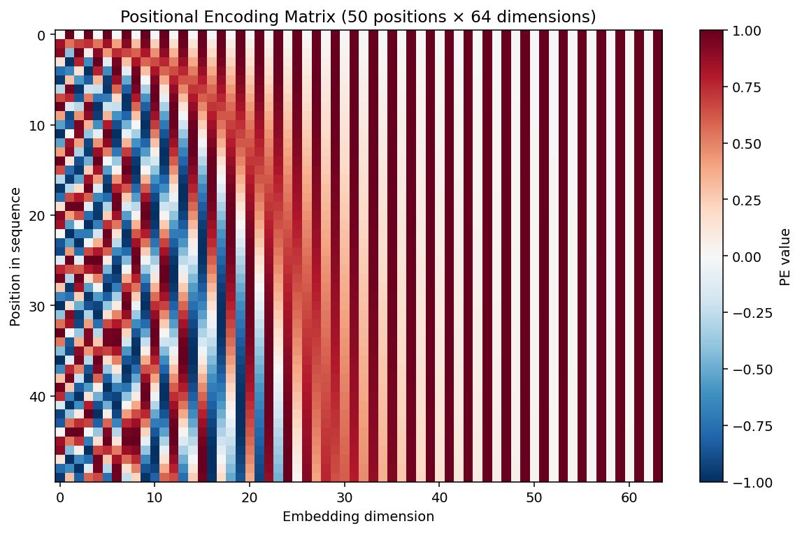
Figure 2: Positional encoding heatmap (50 positions × 64 dimensions).
The wave structure jumps out immediately. The leftmost columns flicker quickly from row to row — those low-index dimensions use the highest frequencies and so distinguish neighbouring positions sharply. The rightmost columns change very slowly from top to bottom — those high-index dimensions use frequencies low enough that nearby positions share nearly identical values, but the slow drift accumulates so that positions hundreds of steps apart still differ. Every row is a unique 64-dim vector — a position fingerprint the network can learn to decode.
Injecting position into the model
With the PE matrix computed and visualised, the final step is to plumb it into the model. Addition is all it takes — one line in the embedding forward pass — and the verification at the end of this section confirms that the symmetry is broken as expected.
To inject this into the model, you simply add the position encoding to the embedded input:
# Reuses MultiHeadAttention (and positional_encoding) defined earlier; assumes top-to-bottom execution.
import torch
import torch.nn as nn

class EmbeddingWithPE(nn.Module):
    def __init__(self, vocab_size, d_model, max_len=512):
        super().__init__()
        self.emb = nn.Embedding(vocab_size, d_model)
        self.register_buffer("pe", positional_encoding(max_len, d_model))

    def forward(self, token_ids):
        # token_ids: (batch, seq_len)
        seq_len = token_ids.size(1)
        return self.emb(token_ids) + self.pe[:seq_len]

emb_layer = EmbeddingWithPE(vocab_size=10000, d_model=64)
token_ids  = torch.randint(0, 10000, (2, 20))
x = emb_layer(token_ids)
print(f"Output shape : {x.shape}")   # (2, 20, 64)
Output:
Output shape : torch.Size([2, 20, 64])The same position vector at position 7 is added to every token that ever sits at position 7, whether the token is "cat", "the", or "hippopotamus". The downstream attention layers now have access to position information and learn to use it.
Let us verify that positional encoding breaks the permutation-equivariance we measured earlier:
# Reuses MultiHeadAttention (and positional_encoding) defined earlier; assumes top-to-bottom execution.
import torch
import torch.nn as nn

torch.manual_seed(0)

class TransformerEmbedding(nn.Module):
    def __init__(self, vocab_size=100, d=128):
        super().__init__()
        self.emb = nn.Embedding(vocab_size, d)
        self.register_buffer("pe", positional_encoding(512, d))
    def forward(self, ids):
        return self.emb(ids) + self.pe[:ids.size(1)]

emb   = TransformerEmbedding()
ids_a = torch.tensor([[5, 3, 8, 1]])           # original order
ids_b = torch.tensor([[8, 5, 1, 3]])           # shuffled

out_a = emb(ids_a)
out_b = emb(ids_b)

# If PE broke equivariance, the outputs should differ even for corresponding tokens
print(f"Token 5 in position 0 vs token 5 in position 1:")
print(f"  Position 0: {out_a[0,0,:4].tolist()}")
print(f"  Position 1: {out_b[0,1,:4].tolist()}")
Output:
Token 5 in position 0 vs token 5 in position 1:
  Position 0: [0.5408, 0.0522, 0.2021, 0.6493]
  Position 1: [1.3822, -0.4075, 0.9639, 0.2972]
Same token 5, different positions, different representations. Positional encoding has broken the symmetry.
Why sine/cosine specifically?
Sine/cosine encoding is elegant, but it is not the only option — and in 2026 it is not even the most common choice. This section maps the landscape of positional encoding variants so that when you see “RoPE” or “ALiBi” in a model card, you know exactly how it relates to what we just built.
Modern variants exist with different trade-offs:
| Variant | Used in | Key property |
|---|---|---|
| Sine/cosine (absolute PE) | Original Transformer | Fixed, zero parameters, generalises theoretically |
| Learned absolute PE | BERT, GPT-2 | Flexible, but cannot generalise to longer sequences |
| RoPE (Rotary PE) | Llama, Qwen, Gemma, Mistral | Applied in attention (not embedding), extrapolates well |
| ALiBi | MPT, BLOOM | Adds bias to attention scores; strong extrapolation |
The original sine/cosine encoding has one beautiful property: any position offset can be expressed as a linear function of any other position. (Vaswani et al. 2017 §3.5: for any offset k, PE(pos+k) can be expressed as a linear function of PE(pos) — equivalently, a 2×2 rotation per frequency pair.) That means the model can in principle learn to generalise to position values it never saw during training, just by composing the position vectors.
For our purposes — building intuition — sine/cosine is the cleanest version. The mechanics of every other variant are basically the same: produce a vector of shape (seq_len, d_model) and add it to the input (or, in the case of RoPE, rotate the Q and K matrices before attention).
Putting it together: the full attention block
All four ingredients are now in hand: an embedding table, positional encoding, and multi-head self-attention. This section assembles them into a single AttentionBlock module — the concrete PyTorch object that prints a parameter count and runs a forward pass you can verify.
We now have everything needed for the attention block used inside every Transformer:
# Reuses MultiHeadAttention (and positional_encoding) defined earlier; assumes top-to-bottom execution.
import torch
import torch.nn as nn

class AttentionBlock(nn.Module):
    """
    Combines positional-encoded embeddings + multi-head self-attention.
    Input: (batch, seq_len) integer token IDs
    Output: (batch, seq_len, d_model) contextualised representations
    """
    def __init__(self, vocab_size, d_model, num_heads, max_len=512):
        super().__init__()
        self.emb_pe = EmbeddingWithPE(vocab_size, d_model, max_len)
        self.mha    = nn.MultiheadAttention(d_model, num_heads, batch_first=True)

    def forward(self, token_ids):
        x = self.emb_pe(token_ids)        # (B, L, d) — embedding + position
        out, _ = self.mha(x, x, x)       # self-attention
        return out

block = AttentionBlock(vocab_size=10000, d_model=128, num_heads=4)
ids   = torch.randint(0, 10000, (2, 16))
out   = block(ids)
print(f"Output shape  : {out.shape}")   # (2, 16, 128)
n = sum(p.numel() for p in block.parameters())
print(f"Parameters    : {n:,}")         # 1,346,048
Output:
Output shape  : torch.Size([2, 16, 128])
Parameters    : 1,346,048
This block is the beating heart of every Transformer. In Part 5, we will wrap it with the residual connections, layer normalization, and feed-forward network that turn it into a full Encoder Layer — the stackable unit that scales to GPT-4’s 96 layers.
MHA parameter count in real models
Having assembled the block, it is instructive to apply the same parameter formula to real architectures so that the numbers you see in model cards become legible. The table below connects what we just built to BERT, GPT-2, and Llama.
With the AttentionBlock above, it is easy to see how attention parameter counts scale across architectures. The four projections (W_Q, W_K, W_V, W_O) each have shape d_model × d_model:
| Model | d_model | Heads | MHA params per layer | Layers | Total MHA params |
|---|---|---|---|---|---|
| BERT-base | 768 | 12 | 4 × 768² = 2.36M | 12 | 28.3M |
| GPT-2 (117M) | 768 | 12 | 4 × 768² = 2.36M | 12 | 28.3M |
| Llama-2-7B (full MHA) | 4096 | 32 | 4 × 4096² = 67.1M | 32 | 2.1B |
| GPT-4 (community estimates; not officially confirmed) | ~12288 | ~96 | 4 × 12288² ≈ 604M | ~96 | ~58B |
In a 7B model like Llama-2-7B, attention parameters are about 2.1B out of 8B total — roughly 26%. (Llama-3-8B uses Grouped-Query Attention with 8 KV heads, so its W_K/W_V projections are 1/4 the size; attention params land closer to ~1.5B on a fully GQA’d model.) The rest is in the FFN layers (Part 5), embeddings, and output heads. This is why LoRA applied to attention projections only (Part 9) captures a large fraction of the task-specific update budget with very few trainable parameters.
Methodology and data sources
Every printed number in this post is captured from a real PyTorch forward pass on a 16 GB CPU-only Mac mini, no GPU. The MultiHeadAttention module uses d_model=128, num_heads=4 (so d_k=32) with default nn.Linear initialization; the permutation-equivariance check uses torch.manual_seed(0) for reproducibility. The positional-encoding matrix is computed with max_len=50, d_model=64 directly from the sine/cosine formulas, and the EmbeddingWithPE and AttentionBlock modules use vocab_size=10000, d_model=128, num_heads=4, max_len=512. No training is needed for this part — the PE matrix is parameter-free, and every shape/parameter count comes from one untrained forward pass.
The sinusoidal positional encoding scheme and the multi-head attention mechanism are both from Vaswani et al., “Attention Is All You Need” (NeurIPS 2017, arXiv:1706.03762). The empirical observations about what individual heads attend to in trained models are from Voita et al., “Analyzing Multi-Head Self-Attention” (ACL 2019, arXiv:1905.09418) and Clark et al., “What Does BERT Look At? An Analysis of BERT’s Attention” (BlackboxNLP 2019, arXiv:1906.04341). The modern positional-encoding variants in the comparison table are: Rotary Position Embedding from Su et al., “RoFormer” (arXiv:2104.09864, 2021), used in Llama, Qwen, Gemma, and Mistral; and ALiBi from Press et al., “Train Short, Test Long” (ICLR 2022, arXiv:2108.12409), used in MPT and BLOOM. The model parameter counts in the comparison table are from the published architecture descriptions in those works’ model cards.
Up next — Part 5: The Transformer Encoder
We now have all the pieces of the original Transformer’s main building block:
- Embeddings (Part 1) and positional encoding (this part) for the input
- Multi-head self-attention (this part) for cross-token information mixing
In Part 5: The Transformer Encoder, we wrap multi-head attention with two more crucial components — residual connections and layer normalization — and add a position-wise feed-forward network. The result is the EncoderLayer, the smallest unit you can repeatedly stack to build a real Transformer. We will build it in PyTorch and look at the actual print(model) output of an 8,544-parameter encoder layer captured from a real run.