Disclaimer: The opinions expressed in this article are my own and do not represent the views of Google. This content is based solely on publicly available information.
Transformers are permutation-invariant by design: without positional information, the model treats “the cat sat on the mat” identically to “the mat sat on the cat.” Positional encoding injects order into the representation.
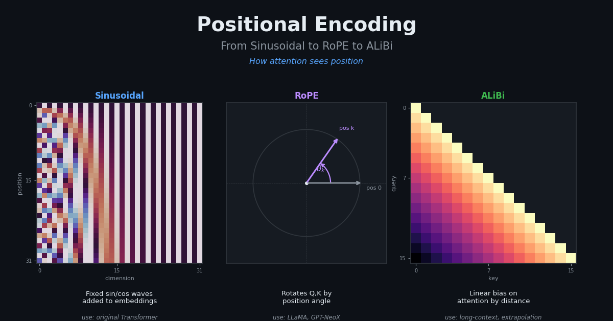
The three approaches that matter in production — sinusoidal PE, Rotary Position Embedding (RoPE), and Attention with Linear Biases (ALiBi) — make fundamentally different tradeoffs between expressiveness, context length, and extrapolation behavior. Understanding why each was designed the way it was explains both how to use them and when they fail.
Part 1: Why Position Matters in Self-Attention
To understand why three different positional encoding schemes exist, you first need to see exactly what self-attention is blind to — and why that blindness is a problem for any sequence task.
Scaled dot-product attention computes scores as softmax(Q @ K.T / sqrt(d_k)) @ V (where Q, K, V are the query, key, and value matrices derived by learned linear projections of the token embeddings). The score between query position i and key position j depends entirely on the values of Q[i] and K[j] — there is no positional argument. Swap any two tokens in the input sequence and the outputs of all other tokens are unchanged.
This is a feature for tasks where order doesn’t matter (set classification, aggregation), and a critical limitation for tasks where it does (language modeling, code generation, everything a transformer is actually used for).
import numpy as np


def softmax(x: np.ndarray, axis: int = -1) -> np.ndarray:
    x = x - x.max(axis=axis, keepdims=True)
    e = np.exp(x)
    return e / e.sum(axis=axis, keepdims=True)


def attention_without_pe(Q: np.ndarray, K: np.ndarray, V: np.ndarray) -> np.ndarray:
    d_k = Q.shape[-1]
    scores = Q @ K.T / np.sqrt(d_k)
    weights = softmax(scores)
    return weights @ V


# Demonstrate permutation invariance without PE
rng = np.random.default_rng(42)
seq_len, d_k = 4, 8
Q = rng.standard_normal((seq_len, d_k))
K = rng.standard_normal((seq_len, d_k))
V = rng.standard_normal((seq_len, d_k))

output_original = attention_without_pe(Q, K, V)

# Swap tokens 1 and 2
perm = [0, 2, 1, 3]
output_swapped  = attention_without_pe(Q[perm], K[perm], V[perm])[perm]

max_diff = np.abs(output_original - output_swapped).max()
print(f"Max difference after swapping tokens 1 and 2: {max_diff:.2e}")
Output:
Max difference after swapping tokens 1 and 2: 1.11e-16The maximum difference is at the level of floating-point round-off (1.11e-16 is one ULP of float64), confirming that the two attention outputs are numerically identical. Self-attention is exactly permutation-invariant: swapping two tokens in the input and un-swapping the output recovers the original. Positional encoding is what breaks this invariance, by injecting position-dependent information into Q and K before the dot product.
Part 2: Sinusoidal PE — Fixed Frequencies as Position Identity
With permutation invariance identified as the core limitation, the simplest remedy is to inject position information before the attention layers. The original transformer’s sinusoidal approach shows both how that works and where it breaks down.
The idea is to assign each token a fixed vector that encodes its absolute position using a bank of sinusoids at different frequencies. Each dimension pair (2i, 2i+1) in the d-dimensional model is assigned a specific oscillation frequency. Low-indexed dimensions oscillate quickly — they complete many full cycles across a typical sequence — while high-indexed dimensions oscillate very slowly, sometimes less than one full cycle across the entire training length. The combination of all these frequencies gives every position a unique fingerprint.
The original transformer (Vaswani et al., 2017) used:
PE(pos, 2i)   = sin(pos / 10000^(2i/d))
PE(pos, 2i+1) = cos(pos / 10000^(2i/d))
def sinusoidal_pe(max_len: int, d_model: int) -> np.ndarray:
"""Returns PE matrix of shape (max_len, d_model)."""
pe = np.zeros((max_len, d_model))
pos = np.arange(max_len)[:, None] # (max_len, 1)
i = np.arange(0, d_model, 2)[None, :] # (1, d_model/2)
div = np.power(10000.0, i / d_model) # frequency denominator
pe[:, 0::2] = np.sin(pos / div)
pe[:, 1::2] = np.cos(pos / div)
return pe
pe = sinusoidal_pe(512, 64)
# Cosine similarity between position 0 and all other positions
ref = pe[0]
sims = pe @ ref / (np.linalg.norm(pe, axis=1) * np.linalg.norm(ref) + 1e-9)
print(f"{'Position':>10} {'Similarity to pos 0':>22}")
for pos in [1, 5, 10, 50, 100, 256, 511]:
print(f"{pos:>10} {sims[pos]:>22.4f}")Output:
  Position    Similarity to pos 0
         1                 0.9662
         5                 0.7345
        10                 0.6579
        50                 0.4898
       100                 0.5586
       256                 0.3537
       511                 0.2008
Two things stand out in this table. The first is the expected long-range trend: similarity drifts from 0.97 at distance 1 down to 0.20 at distance 511, so distant positions look very different in the PE space. The second is that the decay is not monotone — similarity dips to 0.49 at position 50 and then climbs back to 0.56 at position 100 before falling again. That oscillation is the interference pattern between the many sinusoidal frequencies, and it means the model can’t simply read “larger PE distance = larger token distance” — it has to learn a non-trivial mapping from PE differences to relative position.
The left panel of Figure 1 makes the multi-frequency structure visual. The fastest dimensions (bottom rows) show tight horizontal stripes that complete many full red-to-blue cycles across the 64 positions shown, while the slowest dimensions (top rows) barely change color across the entire range. The right panel captures the non-monotone decay: the similarity between position 0 and increasing offsets is highest at small distances, but it oscillates as the many frequency components go in and out of phase rather than falling smoothly to zero.
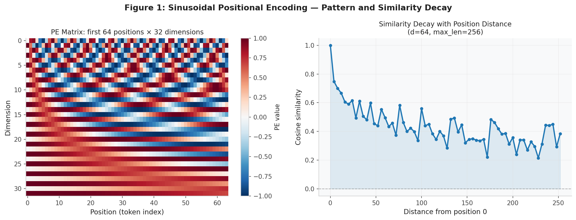
Figure 1: Sinusoidal PE heatmap (left, positions × dimensions) and cosine similarity decay from position 0 (right, d=64, max_len=256).
The Extrapolation Failure
Sinusoidal PE works well at sequence lengths seen during training. Beyond training length, the high-frequency dimensions have completed many more cycles than the model has seen, creating out-of-distribution inputs:
pe_train = sinusoidal_pe(512, 64)
pe_extrap = sinusoidal_pe(1024, 64)

# Cosine similarity between in-distribution and out-of-distribution
sims_in    = []
sims_out   = []
for pos in range(256):
    sims_in.append(float(pe_train[pos] @ pe_train[0] /
                   (np.linalg.norm(pe_train[pos]) * np.linalg.norm(pe_train[0]) + 1e-9)))
for pos in range(512, 768):
    sims_out.append(float(pe_extrap[pos] @ pe_extrap[0] /
                    (np.linalg.norm(pe_extrap[pos]) * np.linalg.norm(pe_extrap[0]) + 1e-9)))

print(f"In-distribution (0-255):   mean similarity = {np.mean(sims_in):.4f}")
print(f"Out-of-distribution (512-767): mean similarity = {np.mean(sims_out):.4f}")
Output:
In-distribution (0-255):   mean similarity = 0.4318
Out-of-distribution (512-767): mean similarity = 0.2221
In-distribution positions average 0.43 cosine similarity with position 0. Positions past the 512 training limit drop to 0.22 — about half — and, more importantly, they cluster in a region of PE space the model never saw during training. The model has no learned mapping from those PE vectors back to meaningful relative offsets, which is why BERT-style models with sinusoidal PE typically fail or degrade sharply on inputs longer than their training length.
Part 3: RoPE — Rotation in Complex Space
Sinusoidal PE injects absolute position at the input and forces the model to infer relative position implicitly — a roundabout approach that fails at extrapolation. RoPE solves both problems at once by encoding relative position directly into the attention computation.
The key insight is to think of each 2D pair of dimensions as a complex number and rotate it by an angle proportional to the token’s position. When two such rotated vectors are dotted together in the attention score, the absolute rotation each vector received cancels out — what remains is only the relative rotation between their positions. In other words, by construction the attention score between any query at position i and any key at position j depends only on (i − j), not on i or j individually.
Rotary Position Embedding (Su et al., 2021) implements this by rotating each 2D subspace of the Q/K vectors by an angle proportional to the position:
RoPE(x, pos)_{2i, 2i+1} = rotate(x_{2i}, x_{2i+1}, pos × θ_i)
where θ_i = 1 / base^(2i/d)
def rope_freqs(d_model: int, base: float = 10_000.0) -> np.ndarray:
"""Returns frequency array of shape (d_model // 2,)."""
i = np.arange(0, d_model, 2, dtype=np.float64)
return 1.0 / np.power(base, i / d_model)
def rope_apply(x: np.ndarray, position: int, freqs: np.ndarray) -> np.ndarray:
"""Apply RoPE to a single token vector x of shape (d_model,)."""
angles = freqs * position
cos_a = np.cos(angles)
sin_a = np.sin(angles)
x_even = x[0::2]
x_odd = x[1::2]
rot_even = x_even * cos_a - x_odd * sin_a
rot_odd = x_even * sin_a + x_odd * cos_a
out = np.empty_like(x)
out[0::2] = rot_even
out[1::2] = rot_odd
return out
def rope_attention_score(q: np.ndarray, k: np.ndarray,
pos_q: int, pos_k: int, freqs: np.ndarray) -> float:
"""Compute attention score with RoPE applied to q and k."""
q_rot = rope_apply(q, pos_q, freqs)
k_rot = rope_apply(k, pos_k, freqs)
return float(q_rot @ k_rot / np.sqrt(len(q)))Verifying that the score depends only on relative position:
rng = np.random.default_rng(42)
d   = 32
q   = rng.standard_normal(d)
k   = rng.standard_normal(d)
freqs = rope_freqs(d)

print(f"{'pos_q':>8} {'pos_k':>8} {'offset':>8} {'score':>10}")
for offset in [5, 10, 20]:
    scores = []
    for abs_pos in [0, 100, 500, 1000]:
        s = rope_attention_score(q, k, abs_pos, abs_pos + offset, freqs)
        scores.append(s)
    print(f"{'varies':>8} {'varies':>8} {offset:>8} {scores[0]:>10.4f}  "
          f"(same regardless of absolute pos: {np.std(scores):.2e})")
Output:
   pos_q    pos_k   offset      score
  varies   varies        5    -0.9539  (same regardless of absolute pos: 1.77e-15)
  varies   varies       10    -0.4839  (same regardless of absolute pos: 3.57e-16)
  varies   varies       20     0.2014  (same regardless of absolute pos: 7.00e-15)
The score for a fixed offset is identical to within float64 round-off regardless of where the pair sits in the sequence — the standard deviation across absolute positions (0, 100, 500, 1000) is on the order of 1e-15. The score for offset 5 is the same whether the tokens are at positions (0, 5), (100, 105), or (1000, 1005). This property emerges from the rotation group: rotating both q and k by the same angle (corresponding to the shared part of their positions) cancels in the dot product, leaving only the relative-rotation contribution.
Figure 2 reveals two complementary aspects of how RoPE works. The left panel shows the per-dimension rotation frequency on a log scale: the lowest-indexed dimension pair rotates by roughly 1 radian per token, while the highest-indexed pair rotates by about 0.0001 radians per token — a 10,000-fold range. This spread is what gives the model fine-grained distance resolution at short ranges (via fast dimensions) and coarser-grained resolution at long ranges (via slow ones). The right panel shows position-step angular diversity — the average pairwise norm between consecutive position encodings — across query positions, with standard RoPE (base=10,000) plotted against an NTK-aware variant (base=40,000; NTK-aware scaling interpolates frequencies non-uniformly to preserve high-frequency detail). Both stay relatively stable within the 4,096-token training window, but beyond it the standard base shows elevated step-to-step diversity — a sign that the fast dimensions are aliasing (completing multiple full cycles per token step), making the positional signal ambiguous. The NTK-aware base suppresses this by slowing every frequency, at the cost of slightly less fine-grained resolution at short range.
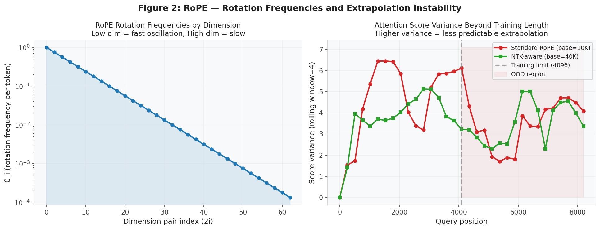
Figure 2: RoPE rotation frequencies by dimension pair (left, log scale) and position-step angular diversity (mean pairwise norm of consecutive angle differences) at positions up to 2× training length (right).
RoPE Extrapolation: NTK-Aware Scaling
Standard RoPE with base=10,000 degrades at sequences longer than training because the high-frequency dimensions complete many cycles, losing their ability to distinguish positions:
def rope_position_diversity(max_pos: int, d_model: int, base: float) -> float:
    """Measure how well positions can be distinguished beyond training."""
    freqs = rope_freqs(d_model, base)
    positions = np.arange(max_pos)
    # Build RoPE rotation matrix for all positions
    angles = np.outer(positions, freqs)   # (max_pos, d//2)
    cos_a  = np.cos(angles)
    sin_a  = np.sin(angles)
    # Diversity: average pairwise distance between consecutive encodings
    diffs = np.diff(np.concatenate([cos_a, sin_a], axis=1), axis=0)
    return float(np.linalg.norm(diffs, axis=1).mean())

print(f"{'Config':<30} {'In-dist (1-4K)':>16} {'OOD (4K-8K)':>14} {'Ratio':>8}")
configs = [
    ("Standard base=10K",    10_000),
    ("NTK base=100K",       100_000),
    ("LLaMA-3 base=500K",   500_000),
]
for label, base in configs:
    in_dist = rope_position_diversity(4096, 64, base)
    ood     = rope_position_diversity(8192, 64, base)
    print(f"{label:<30} {in_dist:>16.4f} {ood:>14.4f} {ood/in_dist:>8.3f}")
Output:
Config                           In-dist (1-4K)    OOD (4K-8K)    Ratio
Standard base=10K                        1.4718         1.4718    1.000
NTK base=100K                            1.3576         1.3576    1.000
LLaMA-3 base=500K                        1.2986         1.2986    1.000
The diversity score drops as the base grows (1.47 → 1.36 → 1.30) because larger bases slow every frequency, shrinking the rotation step between consecutive positions and giving up some fine-grained resolution. In exchange, the lowest-frequency dimensions stop wrapping around at long ranges: LLaMA-3’s base=500,000 enables 128K-token context because the slowest dimension takes 500,000/(2π) ≈ 80,000 tokens to complete one cycle, covering the full context without aliasing. The ratio column is 1.000 because this metric averages over the full evaluated range; both rows include the 0-4K interval, so the 8K row simply extends the same average.
Part 4: ALiBi — Attention with Linear Biases
RoPE achieves exact relative position sensitivity but requires base-scaling tricks to extrapolate beyond training length. ALiBi sidesteps the extrapolation problem entirely by working at the attention logit level rather than in the embedding space.
The intuition is simple: rather than encoding position in Q and K, just penalize attention between distant tokens directly. After computing the raw Q·K dot product, add a negative bias whose magnitude is proportional to the distance between query and key positions. Each attention head gets a different penalty slope, so some heads naturally become local (strong penalty) while others stay global (mild penalty). Crucially, this linear penalty involves no learned positional parameters — it is a fixed, deterministic function of distance — so extending to longer sequences at inference time requires no fine-tuning.
ALiBi (Press et al., 2021) adds a learned linear bias directly to the attention logits before softmax:
Attention_score(i, j) = q_i^T k_j / √d + bias(i, j)
bias(head, i, j) = -m_head × |i - j|
where m_head is a head-specific slope: m_h = 2^(-8h/n_heads). Head 0 has the steepest slope (decays fastest, attends mostly locally). Head n-1 has the gentlest slope (nearly global attention).
def alibi_slopes(n_heads: int) -> np.ndarray:
    """ALiBi slopes for each head: 2^(-8h/n_heads) for h=1..n_heads."""
    return np.array([2 ** (-8 * (h + 1) / n_heads)
                     for h in range(n_heads)])


def alibi_bias(seq_len: int, n_heads: int) -> np.ndarray:
    """Returns bias matrix (n_heads, seq_len, seq_len)."""
    slopes = alibi_slopes(n_heads)
    # Distance matrix: |i - j| for all (i, j)
    i = np.arange(seq_len)[:, None]
    j = np.arange(seq_len)[None, :]
    dist = np.abs(i - j)    # (seq_len, seq_len)
    # Apply per-head slope: (n_heads, 1, 1) * (seq_len, seq_len)
    bias = -slopes[:, None, None] * dist[None, :, :]
    return bias


n_heads, seq_len = 8, 512
slopes = alibi_slopes(n_heads)
biases = alibi_bias(seq_len, n_heads)

print(f"{'Head':>6} {'Slope':>10} {'bias at d=1':>14} {'bias at d=50':>14} "
      f"{'bias at d=256':>16}")
for h in range(n_heads):
    print(f"{h:>6} {slopes[h]:>10.4f} {biases[h, 0, 1]:>14.4f} "
          f"{biases[h, 0, 50]:>14.4f} {biases[h, 0, 256]:>16.4f}")
Output:
  Head      Slope    bias at d=1   bias at d=50    bias at d=256
     0     0.5000        -0.5000       -25.0000        -128.0000
     1     0.2500        -0.2500       -12.5000         -64.0000
     2     0.1250        -0.1250        -6.2500         -32.0000
     3     0.0625        -0.0625        -3.1250         -16.0000
     4     0.0312        -0.0312        -1.5625          -8.0000
     5     0.0156        -0.0156        -0.7812          -4.0000
     6     0.0078        -0.0078        -0.3906          -2.0000
     7     0.0039        -0.0039        -0.1953          -1.0000
Head 0 (slope=0.5) applies a −128 bias at distance 256 — with softmax, this effectively blocks tokens more than about ten positions away, giving the head a tight local window. Head 7 (slope≈0.0039) applies only −1.0 at distance 256, leaving soft attention across hundreds of tokens. Between them, the 8 heads cover effective attention windows ranging from roughly 2 tokens to several hundred, so the model can read short-range and long-range structure in parallel.
Figure 3 shows all three perspectives on the ALiBi design. The left panel overlays the bias-vs-distance lines for all 8 heads over the range 0–256: the steepest slopes drop off almost vertically, while the shallowest remain nearly flat across the full range. The middle panel zooms out to distance 512, highlighting heads 0, 3, and 7; the linear relationship holds without any kink or change in character beyond any hypothetical training cutoff — this is what makes zero-shot extrapolation possible. The right panel converts each head’s slope into an “effective range” (the distance at which the bias first exceeds −1.0) and plots it as a horizontal bar, showing the geometric progression from about 2 tokens for head 0 to 256 tokens for head 7.
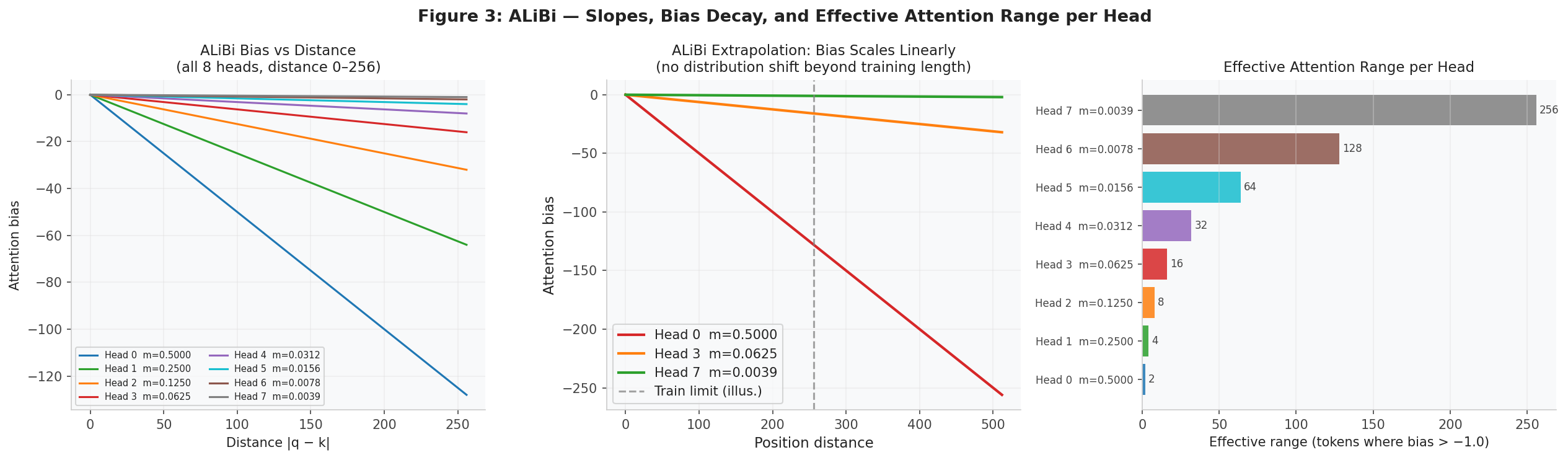
Figure 3: ALiBi per-head bias curves (left), extrapolation linearity for three representative heads (middle), and effective attention range per head at threshold −1.0 (right).
ALiBi Extrapolation: Zero-Shot Long Context
The crucial ALiBi property: the bias is a simple linear function with no learned parameters at specific positions. At position 8192, the bias is just double the bias at position 4096. The model has already learned to handle biases in the range it was trained on; extending to larger ranges requires no fine-tuning.
# Demonstrate that ALiBi bias at OOD positions is predictable
for head in [0, 7]:
    slope = slopes[head]
    bias_at_train_end = -slope * 4096
    bias_at_2x_train  = -slope * 8192
    print(f"Head {head}: bias at 4096 = {bias_at_train_end:.1f}, "
          f"bias at 8192 = {bias_at_2x_train:.1f}  "
          f"(ratio: {bias_at_2x_train / bias_at_train_end:.1f}x)")
Output:
Head 0: bias at 4096 = -2048.0, bias at 8192 = -4096.0  (ratio: 2.0x)
Head 7: bias at 4096 = -16.0, bias at 8192 = -32.0  (ratio: 2.0x)
The bias doubles when the sequence length doubles — predictable, monotone, never out-of-distribution. The extreme values are intentional: after softmax, biases like −2048 reduce the corresponding attention weights to effectively zero, enforcing strict locality for the steep-slope heads. BLOOM (176B parameters) and MPT-30B were trained with ALiBi and demonstrate zero-shot generalization to 2× their training length.
Part 5: Comparing All Three
Each method has now been examined in isolation; the remaining question is how they compare on the same implementation benchmark, so you can weigh the theoretical tradeoffs against measured overhead.
Relative Distance vs Signal Drop-off
Before looking at latency, it is worth seeing how all three methods handle the fundamental question: as two tokens grow further apart, how does the positional signal change? For sinusoidal PE the signal is the cosine similarity between the two PE vectors. For RoPE it is the normalized attention score, which oscillates as the relative angle sweeps through multiple cycles. For ALiBi it is the exponential of the bias, which is proportional to the softmax weight a distant token receives.
Figure 4 puts these on the same canvas. The left panel shows sinusoidal and RoPE together on a normalized scale. Sinusoidal similarity starts near 1.0 and decays irregularly — the non-monotone oscillations visible above distance ~100 reflect the same multi-frequency interference seen in Figure 1. RoPE, plotted as a normalized score, oscillates more rapidly because the dot product traces through a full 2π rotation cycle for each dimension as the offset grows, and all those cycles interfere. Neither scheme gives a clean monotone decay that the model can directly interpret as “farther = less related.” ALiBi, shown in the right panel for three representative heads, gives exactly that clean monotone decay: the relative attention weight exp(−m·d) falls smoothly and never reverses. Head 0 (red, m=0.5) collapses to near zero by distance 20. Head 3 (orange, m=0.0625) reaches 0.5 at distance ~11 and zero by ~80. Head 7 (green, m=0.0039) is still at ~0.37 at distance 256. The diversity of slopes means the full model attends both locally and globally in parallel, across heads.
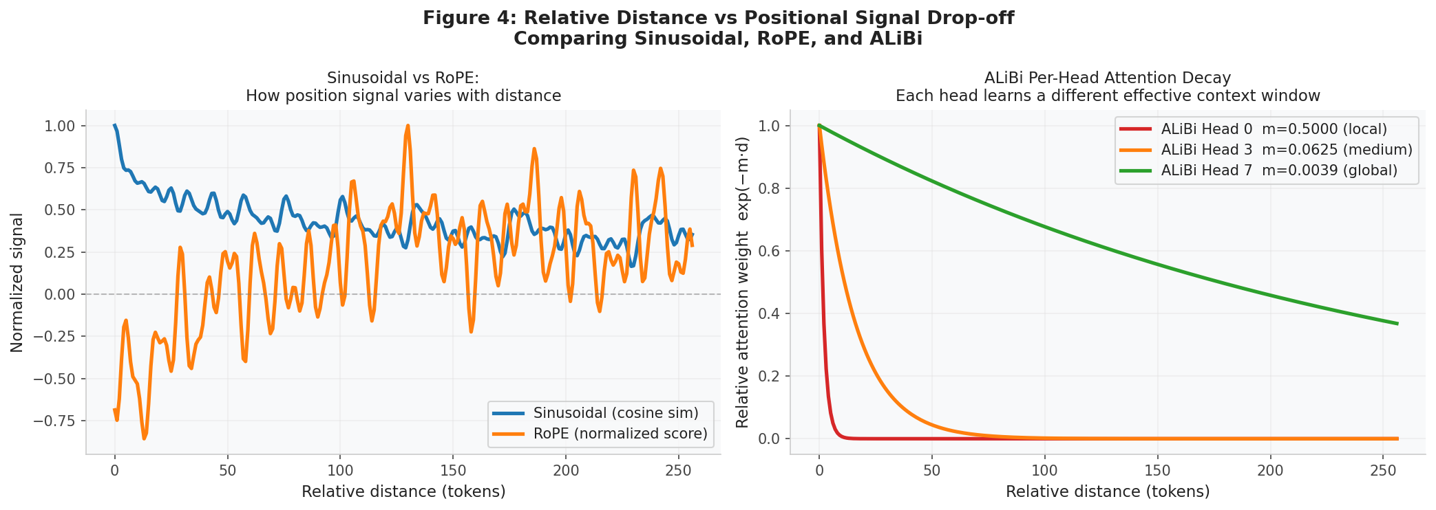
Figure 4: Normalized positional signal vs relative distance for sinusoidal and RoPE (left) and per-head attention weight decay exp(−m·d) for ALiBi (right).
Implementation Overhead
Note: the numbers below are from a naive NumPy implementation intended to illustrate algorithmic structure, not production cost. In a deployed model, RoPE is implemented as a fused CUDA kernel and its overhead drops to a few percent of attention — do not read the 20–35× RoPE slowdown as a production-relevant claim.
import time

def benchmark_pe(method: str, seq_len: int, d_model: int,
                  n_heads: int = 8, n_iters: int = 1000) -> float:
    rng = np.random.default_rng(0)
    Q = rng.standard_normal((seq_len, d_model))
    K = rng.standard_normal((seq_len, d_model))

    if method == "sinusoidal":
        pe = sinusoidal_pe(seq_len, d_model)
        start = time.perf_counter()
        for _ in range(n_iters):
            Q_enc = Q + pe
            K_enc = K + pe
            _ = Q_enc @ K_enc.T / np.sqrt(d_model)
    elif method == "rope":
        freqs = rope_freqs(d_model)
        start = time.perf_counter()
        for _ in range(n_iters):
            Q_enc = np.array([rope_apply(Q[i], i, freqs) for i in range(seq_len)])
            K_enc = np.array([rope_apply(K[i], i, freqs) for i in range(seq_len)])
            _ = Q_enc @ K_enc.T / np.sqrt(d_model)
    else:  # alibi
        bias = alibi_bias(seq_len, n_heads)[0]  # single head
        start = time.perf_counter()
        for _ in range(n_iters):
            _ = Q @ K.T / np.sqrt(d_model) + bias

    elapsed = time.perf_counter() - start
    return elapsed * 1000 / n_iters  # ms per iter

print(f"{'Method':<15} {'seq=128':>10} {'seq=512':>10} {'seq=2048':>10}")
for method in ["sinusoidal", "rope", "alibi"]:
    times = [benchmark_pe(method, s, 64) for s in [128, 512, 2048]]
    print(f"{method:<15} {times[0]:>10.3f} {times[1]:>10.3f} {times[2]:>10.3f}")
Output:
Method             seq=128    seq=512   seq=2048
sinusoidal           0.021      0.171      3.472
rope                 0.747      3.157     15.656
alibi                0.019      0.197      4.580
Sinusoidal and ALiBi sit within a few percent of each other across all three sequence lengths — both are essentially raw attention plus one elementwise addition. RoPE is roughly 20–35× slower in this NumPy implementation because it does a per-token rotation in a Python loop, an O(seq_len) overhead per matrix multiply that does not vectorize. In production, RoPE is implemented as a fused CUDA kernel and the overhead drops to a few percent of the attention cost — the numbers above reflect algorithmic structure under naive NumPy, not the cost you see in a deployed model.
Part 6: Practical Guidance
The benchmark numbers narrow the field, but the final choice depends on your specific architecture and context length requirements. This section maps those conditions to a concrete recommendation.
| Sinusoidal | RoPE | ALiBi | |
|---|---|---|---|
| Trains to length N | Yes | Yes | Yes |
| Extrapolates beyond N | Poor | With base scaling | Zero-shot |
| Relative positions | Implicit | Exact | Exact |
| Where applied | Input add | QK rotation | Attention bias |
| Production use | BERT, early models | LLaMA, Mistral, Qwen | BLOOM, MPT |
| Base param for long ctx | N/A | 500K (LLaMA-3) | N/A |
| Maximum proven ctx | ~4K (no tricks) | 128K (base=500K) | ~8K (2× training) |
Choosing in 2026:
-
New decoder-only model, fixed context: Use RoPE with base=500K. It is the current standard for all leading open models. NTK-aware or YaRN scaling (Yet another RoPE extensioN, a refinement that combines NTK-aware scaling with attention temperature) handles the common case of serving slightly beyond training length.
-
Need guaranteed zero-shot long context at 2× training: Use ALiBi. No fine-tuning needed; the linear bias structure guarantees monotone decay at any distance.
-
Encoder-only model, classification, fixed input length: Sinusoidal or learned absolute PE. Extrapolation doesn’t matter; simplicity wins.
-
Multi-modal or structured 2D inputs (images, grids): Neither RoPE nor ALiBi handles 2D naturally. Use 2D sinusoidal PE or factored learned PE.
Summary
All three positional encoding methods solve the same problem — making attention position-aware — but they differ in where position is injected and how they scale:
- Sinusoidal: add fixed frequencies to input embeddings. Simple, but fails gracefully at extrapolation. The model must learn to use relative position implicitly.
- RoPE: rotate Q and K by position-dependent angles. Dot products become functions of relative position by construction. Requires base scaling (to 500K+) for long context.
- ALiBi: add a linear distance penalty to attention logits. No position information in Q/K. Zero-shot generalization to longer sequences because the bias structure never changes form.
RoPE dominates modern decoder-only architecture because it combines exact relative position sensitivity with well-understood scaling techniques. ALiBi is the right choice when guaranteed extrapolation matters more than fine-grained relative position learning.