Disclaimer: The opinions expressed in this article are my own and do not represent the views of Google. This content is based solely on publicly available information.
Every practitioner working with transformers has encountered the attention mechanism described the same way: “it lets tokens attend to each other.” That description is accurate and useless. It says nothing about why the mechanism works, what it is computing, or why the specific design choices — scaled dot-product, multi-head, the square-root denominator — are not arbitrary.
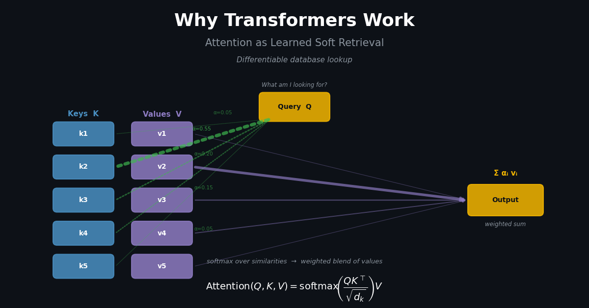
The cleaner mental model: attention is a differentiable database lookup. You have a set of key-value pairs stored in the sequence, and a query. Attention computes a weighted retrieval over all values, where the weights are determined by how well each key matches the query. Make the retrieval differentiable and you can train it end-to-end. Make the keys and values learned projections and the model can decide what information to store and retrieve. That is the entire mechanism.
This article builds that model from first principles — from the raw matrix operations, through multi-head design, to the quadratic scaling problem that modern architectures exist to solve. It also connects attention to classical associative memory (Hopfield networks), which clarifies why the mechanism has exponential storage capacity rather than the polynomial capacity of its predecessor.
The Retrieval View
A traditional database lookup is hard: you provide an exact key, you get back the matching value or nothing. Attention replaces the hard lookup with a soft one. Every key in the database contributes to the output, weighted by how well it matches the query. The weights are non-negative and sum to one, so the output is a convex combination of all values.
Formally, given a query vector Q, key matrix K, and value matrix V (one row per token):
Attention(Q, K, V) = softmax(Q @ K.T / sqrt(d_k)) @ VThe Q @ K.T term computes a dot-product similarity between the query and every key. Dividing by sqrt(d_k) keeps the dot products in a stable range regardless of embedding dimension — without this, large d_k values cause dot products to grow large, softmax saturates to near-one-hot, and gradients vanish. The softmax turns similarities into a probability distribution, and multiplying by V computes the weighted retrieval.
Here is the full implementation with no dependencies beyond NumPy. Q, K, V are themselves produced by X @ W_Q, X @ W_K, X @ W_V — the multi-head section below shows this explicitly. We treat them as inputs here to keep the soft-retrieval mechanism front and center.
from __future__ import annotations
import numpy as np


def softmax(x: np.ndarray, axis: int = -1) -> np.ndarray:
    x = x - x.max(axis=axis, keepdims=True)
    e = np.exp(x)
    return e / e.sum(axis=axis, keepdims=True)


def scaled_dot_product_attention(
    Q: np.ndarray,   # (seq_len, d_k)
    K: np.ndarray,   # (seq_len, d_k)
    V: np.ndarray,   # (seq_len, d_v)
    mask: np.ndarray | None = None,
    temperature: float = 1.0,
) -> tuple[np.ndarray, np.ndarray]:
    """Returns (output, attention_weights). Output shape: (seq_len, d_v)."""
    d_k = Q.shape[-1]
    scale = np.sqrt(d_k) * temperature
    scores = Q @ K.T / scale
    if mask is not None:
        scores = scores + mask    # additive mask; large negative → 0 after softmax
    weights = softmax(scores, axis=-1)
    output = weights @ V
    return output, weights
The temperature parameter generalises the standard formulation. temperature=1.0 is the classic scaled dot-product. Lower temperature sharpens attention toward the best-matching key; higher temperature flattens it toward uniform.
Running this on a six-token sentence produces the following attention weights:
import warnings
import numpy as np
warnings.filterwarnings("ignore", category=RuntimeWarning)

rng = np.random.default_rng(0)
seq_len, d_k = 6, 8
Q = rng.standard_normal((seq_len, d_k))
K = rng.standard_normal((seq_len, d_k))
V = rng.standard_normal((seq_len, d_k))

_, weights = scaled_dot_product_attention(Q, K, V)
print(f"  {'Token':>8} {'Peak attends to':>18} {'Max weight':>12} {'Entropy (nats)':>16}")
for i, row in enumerate(weights):
    peaked = np.argmax(row)
    print(f"  {i:>8} {peaked:>18} {row[peaked]:>12.3f} "
          f"{-np.sum(row*np.log(row+1e-9)):>16.3f}")
Output:
     Token   Peak attends to   Max weight  Entropy (nats)
         0                 3        0.352           1.641
         1                 4        0.414           1.612
         2                 3        0.269           1.675
         3                 0        0.461           1.483
         4                 5        0.290           1.697
         5                 5        0.519           1.323
Each token attends most strongly to one other token, but distributes weight across all of them. The entropy column quantifies how spread out the attention is — higher entropy means more uniform, lower means more peaked. This is the key difference from hard lookup: every token participates in every output, just at different weights.
The heatmap visualisation makes the soft-lookup structure explicit. Each row is one query token, each column is one key token, and the colour intensity is the attention weight. No cell is empty: every token contributes to every output, just at different strengths. Some rows concentrate most of their mass on one or two columns; others spread weight more evenly — that variation in row sparsity is exactly the “soft” part of soft retrieval. The bar chart on the right collapses each row to its strongest link, which is the closest analogue to a hard-lookup result.
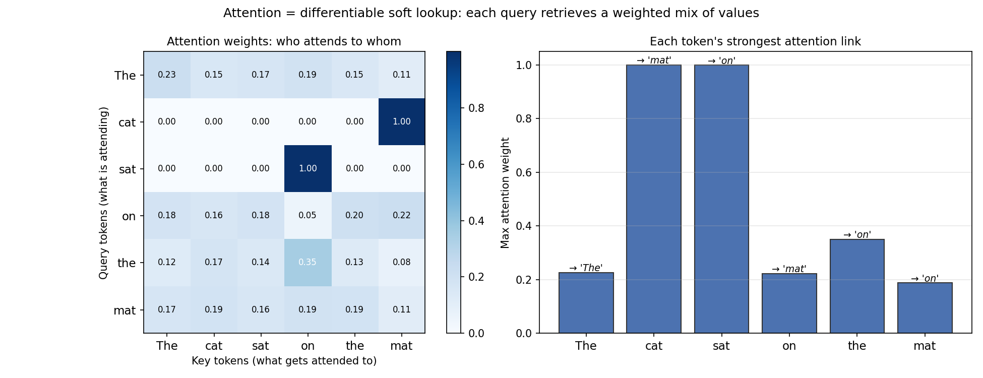 Figure 1: Attention weights as a soft lookup table.
Softmax Temperature and Attention Sharpness
The soft-lookup framing raises an immediate question: how soft is “soft”? The answer lies in the temperature implicit in the scaling term. The sqrt(d_k) scaling in the denominator plays a specific role: it keeps dot products from growing with embedding dimension. But the softmax has a second implicit parameter — its temperature. When you replace sqrt(d_k) with sqrt(d_k) * T, you control how sharply or broadly the model distributes attention.
print(f"  {'Temperature':>12} {'Mean entropy (nats)':>22} {'Mean max weight':>18}")
for T in [0.25, 0.5, 1.0, 2.0, 4.0]:
    _, w = scaled_dot_product_attention(Q, K, V, temperature=T)
    entropy = float(np.mean(-np.sum(w * np.log(w + 1e-9), axis=-1)))
    max_w = float(np.mean(w.max(axis=-1)))
    print(f"  {T:>12.2f} {entropy:>22.4f} {max_w:>18.4f}")
Output:
   Temperature    Mean entropy (nats)    Mean max weight
          0.25                 0.7926             0.7024
          0.50                 1.4007             0.5019
          1.00                 1.8555             0.3072
          2.00                 2.0147             0.2066
          4.00                 2.0613             0.1629
At T=0.25, the mean maximum weight is 0.70 — the model almost performs hard lookup. At T=4.0, the maximum weight drops to 0.16, barely above uniform (1/6 ≈ 0.167 for 6 tokens). The entropy tells the same story: low temperature means low entropy (concentrated), high temperature means high entropy (spread).
This is not just theoretical. In trained transformers, early layers tend to have broader attention (higher effective temperature) because they need to gather context. Late layers tend to be sharper (lower effective temperature) because they have already composed information and are selecting specific components. The model learns this implicitly through the learned Q, K, V projection matrices — there is no explicit temperature knob, only the effective scale of the learned weights.
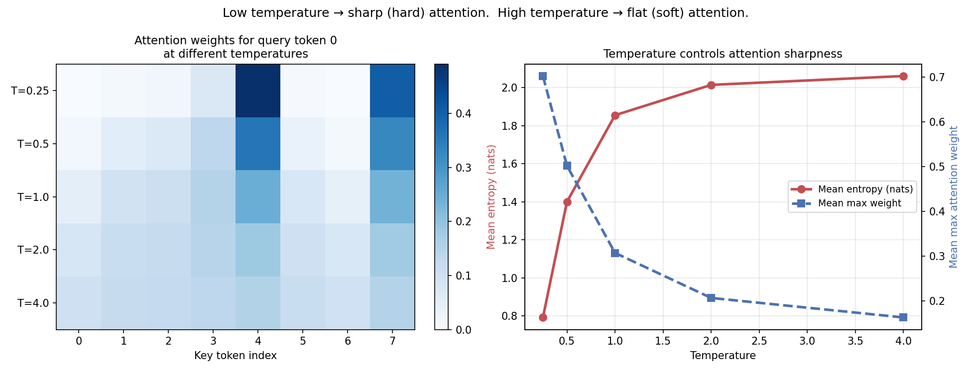 Figure 2: Temperature controls the sharpness of the soft lookup.
Multi-Head Attention: Parallel Subspace Projections
A single soft lookup is expressive, but it can only encode one retrieval pattern at a time — one notion of “what to attend to.” Real language requires many such notions operating simultaneously: attending to the nearest noun phrase, the subject of the sentence, or the pronoun antecedent, all at once. Multi-head attention solves this by running H independent attention heads in parallel, each with its own learned Q, K, V projection matrices, then concatenating and projecting the results.
# Multi-head attention: H independent lookups in parallel subspaces
def multi_head_attention(
    X: np.ndarray,    # (seq_len, d_model)
    W_Q: np.ndarray,  # (n_heads, d_model, d_k)
    W_K: np.ndarray,  # (n_heads, d_model, d_k)
    W_V: np.ndarray,  # (n_heads, d_model, d_v)
    W_O: np.ndarray,  # (n_heads * d_v, d_model)
) -> tuple[np.ndarray, np.ndarray]:
    """Returns (output, all_head_weights). output shape: (seq_len, d_model)."""
    n_heads = W_Q.shape[0]
    head_outputs = []
    all_weights = []
    for h in range(n_heads):
        Q = X @ W_Q[h]   # (seq_len, d_k)
        K = X @ W_K[h]
        V = X @ W_V[h]
        out, w = scaled_dot_product_attention(Q, K, V)
        head_outputs.append(out)
        all_weights.append(w)
    concat = np.concatenate(head_outputs, axis=-1)  # (seq_len, n_heads * d_v)
    output = concat @ W_O                           # (seq_len, d_model)
    return output, np.stack(all_weights)            # weights: (n_heads, seq, seq)
The projection matrices W_Q[h], W_K[h], W_V[h] are shape (d_model, d_k) where d_k = d_model / n_heads. Each head operates in a lower-dimensional subspace of the full embedding. This is not a computational trick to reduce cost — it is the mechanism by which different heads learn different things. Head 0’s Q projection matrix defines what “asking about” means in its subspace; head 1’s defines something different. The output projection W_O then combines all heads back into the full d_model space.
Running four heads on the same sequence:
rng = np.random.default_rng(42)
seq_len, d_model, n_heads = 8, 32, 4
d_k = d_v = d_model // n_heads

X = rng.standard_normal((seq_len, d_model))
W_Q = rng.standard_normal((n_heads, d_model, d_k)) * 0.1
W_K = rng.standard_normal((n_heads, d_model, d_k)) * 0.1
W_V = rng.standard_normal((n_heads, d_model, d_v)) * 0.1
W_O = rng.standard_normal((n_heads * d_v, d_model)) * 0.1

_, all_weights = multi_head_attention(X, W_Q, W_K, W_V, W_O)
print(f"  {'Head':>6} {'Peak token (avg)':>18} {'Mean entropy':>14} {'Agreement w/ head 0':>22}")
ref = all_weights[0]
for h in range(n_heads):
    w = all_weights[h]
    avg_peak = float(np.mean(np.argmax(w, axis=-1)))
    entropy = float(np.mean(-np.sum(w * np.log(w + 1e-9), axis=-1)))
    agreement = float(np.mean(np.sum(ref * w, axis=-1)))
    print(f"  {h:>6} {avg_peak:>18.2f} {entropy:>14.4f} {agreement:>22.4f}")
Output:
    Head   Peak token (avg)   Mean entropy    Agreement w/ head 0
       0               5.25         2.0457                 0.1331
       1               2.38         2.0454                 0.1265
       2               2.75         2.0490                 0.1264
       3               4.12         2.0378                 0.1254
Each head peaks on different tokens on average (5.25 vs 2.38 vs 2.75 vs 4.12), and the agreement between heads is low (0.125–0.133, barely above uniform for 8 tokens). These are random initialization results — trained heads diverge even further, each specialising in patterns the gradient has found useful. Mechanistic interpretability work on production models has found heads that consistently track specific syntactic relations (previous-token heads, induction heads that copy from earlier occurrences) and others that pool global context onto a “BOS (Beginning Of Sequence token)“-like sink token.
The multi-head panel below makes the diversity concrete. Each head’s projection matrices are independent random draws, so each head ends up scoring the same input through a different similarity geometry. The resulting heatmaps look visibly different — different rows peak in different columns, different rows concentrate versus spread, and the bright cells line up differently across heads. The point is that several heads sharing input and architecture nonetheless express distinct retrieval patterns, which after training is what lets each head specialise.
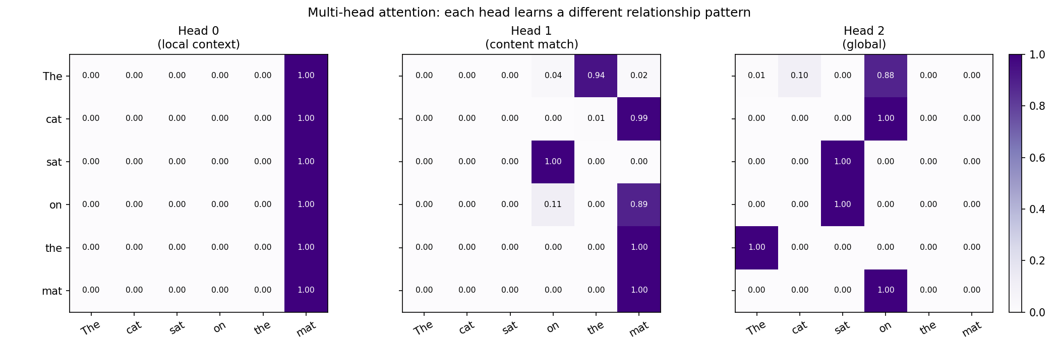 Figure 3: Four heads on the same input, four different retrieval patterns.
Causal Masking: Preventing Future Leakage
Multi-head attention as described so far is bidirectional — every token can attend to every other. For autoregressive generation, that would let the model read tokens it has not yet produced. Causal masking is the mechanism that enforces left-to-right generation order. Encoder-only transformers (BERT (Bidirectional Encoder Representations from Transformers)) use full bidirectional attention — each token can attend to every other token. Decoder-only transformers (GPT (Generative Pre-trained Transformer)-family) use causal attention — at position i, the model can only attend to positions 0..i. Without this constraint, the model would read the answer before generating it.
The implementation uses an additive mask: fill future positions with a large negative value, which becomes near-zero after softmax.
# Causal mask: large negative values in future positions become near-zero after softmax
def causal_mask(seq_len: int) -> np.ndarray:
    """Upper-triangular mask (future tokens set to -inf)."""
    mask = np.zeros((seq_len, seq_len))
    mask[np.triu_indices(seq_len, k=1)] = -1e9
    return mask
Verify that no future weight leaks through:
seq_len, d_k = 5, 8
Q = rng.standard_normal((seq_len, d_k))
K = rng.standard_normal((seq_len, d_k))
V = rng.standard_normal((seq_len, d_k))
mask = causal_mask(seq_len)

_, w = scaled_dot_product_attention(Q, K, V, mask=mask)
for i, row in enumerate(w):
    future_sum = float(row[i+1:].sum())
    print(f"  token {i}: weights={np.round(row, 3)}  future_leak={future_sum:.6f}")
Output:
  token 0: weights=[1. 0. 0. 0. 0.]  future_leak=0.000000
  token 1: weights=[0.67 0.33 0.   0.   0.  ]  future_leak=0.000000
  token 2: weights=[0.317 0.509 0.175 0.    0.   ]  future_leak=0.000000
  token 3: weights=[0.575 0.188 0.117 0.12  0.   ]  future_leak=0.000000
  token 4: weights=[0.051 0.274 0.266 0.168 0.242]  future_leak=0.000000
Token 0 can only attend to itself (weight = 1.0). Token 4 attends to all five tokens. Future leak is exactly zero. The additive mask approach is numerically equivalent to zeroing out future positions and more stable than multiplying by a binary mask, because the subtraction happens before softmax rather than after.
The Quadratic Scaling Problem
The mechanism works — but it comes with a cost that does not scale gracefully. The score matrix Q @ K.T has shape (seq_len, seq_len). For a sequence of length n, this is O(n²) in both compute and memory. Everything else in the attention layer scales linearly.
To make this concrete, the function below computes the total FLOPs (floating-point operations) and score-matrix memory for a single attention layer. The QKV projection step is linear in sequence length; the score computation and weighted sum are both quadratic — those two quadratic terms dominate at longer contexts.
# FLOPs and score-matrix memory as a function of sequence length
def attention_complexity(seq_len: int, d_model: int) -> dict[str, int]:
    d_k = d_model
    qkv_flops = 3 * seq_len * d_model * d_k     # QKV projections
    score_flops = seq_len * seq_len * d_k        # score matrix
    wsum_flops = seq_len * seq_len * d_k         # weighted sum
    return {
        "seq_len": seq_len,
        "flops": qkv_flops + score_flops + wsum_flops,
        "score_memory": seq_len * seq_len,       # float32 elements
    }
Running this across context lengths with d_model=512:
print(f"  {'seq_len':>10} {'FLOPs':>14} {'Score matrix (MB)':>20}")
for seq in [128, 512, 1024, 4096, 16384, 65536]:
    c = attention_complexity(seq, 512)
    mem_mb = c["score_memory"] * 4 / (1024 ** 2)
    print(f"  {seq:>10,} {c['flops']:>14,} {mem_mb:>20.1f}")
Output:
     seq_len          FLOPs    Score matrix (MB)
         128    117,440,512                  0.1
         512    671,088,640                  1.0
       1,024  1,879,048,192                  4.0
       4,096 20,401,094,656                 64.0
      16,384 287,762,808,832               1024.0
      65,536 4,449,586,118,656              16384.0
At 4,096 tokens, the score matrix alone occupies 64 MB per layer per head — multiply by 32 layers and 32 heads and you are at roughly 64 GB just for score matrices (64 MB × 32 layers × 32 heads = 65,536 MB ≈ 64 GB), before weights, activations, or gradients. At 65,536 tokens, the score matrix is 16 GB per head. This is why the transformer architecture that dominated 2018–2022 cannot naively scale to 100K+ context lengths, and why Flash Attention (which tiles the score matrix computation to avoid materializing the full matrix), sliding-window attention, and linear attention approximations exist.
The two bar charts below visualise the cost curve from 128 to 16,384 tokens. Both compute and score-matrix memory grow as O(n²), so doubling the context quadruples both. The bars below 4K (blue) stay within a regime that fits comfortably in GPU L2 cache and a few hundred MB of HBM (High Bandwidth Memory — the GPU’s main DRAM). The bars at and above 4K (red) cross into territory where the score matrix dominates total memory and forces architectural workarounds.
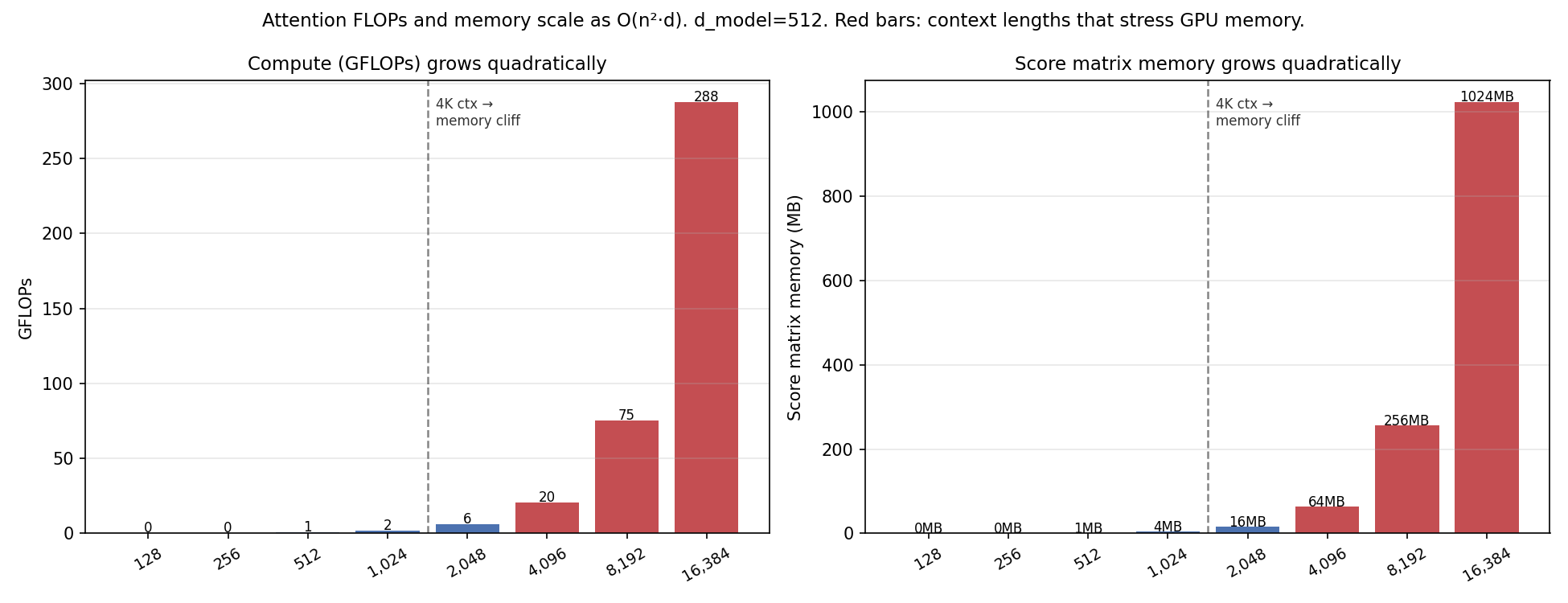 Figure 4: Attention compute and score-matrix memory both scale as O(n²) in both compute and memory (with a per-head
 d_k factor in compute).
Connection to Hopfield Networks
The soft-retrieval framing is not just a useful analogy — it has a formal mathematical grounding in associative memory theory. Understanding this connection explains why attention scales to rich, high-dimensional sequences without saturating. The classical Hopfield network (1982) is a content-addressable memory: store binary patterns as attractors in a weight matrix, then retrieve them by starting from a noisy query and iterating to convergence. It has linear capacity: roughly 0.14 × N patterns for a network with N neurons.
from __future__ import annotations
import numpy as np


class ClassicalHopfield:
    """Hopfield network trained with Hebbian learning on bipolar (+1/-1) patterns."""

    def __init__(self, n: int):
        self.n = n
        self.W = np.zeros((n, n))

    def store(self, patterns: np.ndarray) -> None:
        for p in patterns:
            self.W += np.outer(p, p) / self.n
        np.fill_diagonal(self.W, 0)

    def retrieve(self, query: np.ndarray, n_iters: int = 20) -> np.ndarray:
        state = np.sign(query).astype(float)
        state[state == 0] = 1.0
        for _ in range(n_iters):
            new_state = np.sign(self.W @ state)
            new_state[new_state == 0] = 1.0
            if np.array_equal(new_state, state):
                break
            state = new_state
        return state
The modern Hopfield network (Ramsauer et al., 2020) replaces the Hebbian weight matrix and binary state update with a continuous exponential interaction function. The update rule becomes:
state_new = X_stored.T @ softmax(β * X_stored @ query)Recognise this? It is exactly scaled dot-product attention where the query is query, the keys are X_stored, the values are X_stored, and β plays the role of 1/sqrt(d_k) — i.e., setting β = 1/√d_k recovers the scaled dot-product attention formula softmax(Q·K^T / √d_k)·V. The formal equivalence — proved in the paper — shows that attention is a one-step modern Hopfield update. The payoff: modern Hopfield networks have exponential storage capacity rather than linear.
class ModernHopfield:
    """Continuous Hopfield network — one-step retrieval, exponential capacity."""

    def __init__(self, beta: float = 1.0):
        self.beta = beta
        self.X: np.ndarray | None = None

    def store(self, patterns: np.ndarray) -> None:
        self.X = patterns

    def retrieve(self, query: np.ndarray) -> np.ndarray:
        assert self.X is not None
        logits = self.beta * self.X @ query
        logits -= logits.max()
        weights = np.exp(logits)
        weights /= weights.sum()
        return self.X.T @ weights
rng = np.random.default_rng(0)
# Classical Hopfield uses bipolar (+1/-1) patterns; modern uses continuous.
bipolar = rng.choice([-1.0, 1.0], size=(200, 64)) # 200 patterns, n=64
patterns = rng.standard_normal((200, 64)) # continuous patterns
target_bipolar = bipolar[0]
target_cont = patterns[0]
noisy_bipolar = target_bipolar.copy()
noisy_bipolar[rng.choice(64, 6, replace=False)] *= -1 # flip 6 bits
noisy_cont = target_cont + 0.3 * rng.standard_normal(64)
classical = ClassicalHopfield(n=64)
classical.store(bipolar[:9]) # ~0.14·n ≈ 9 patterns capacity
modern = ModernHopfield(beta=1.0)
modern.store(patterns) # exponential capacity in d
classical_ok = np.array_equal(classical.retrieve(noisy_bipolar), target_bipolar)
modern_ok = np.allclose(modern.retrieve(noisy_cont), target_cont, atol=0.3)
print(f"Classical (9 patterns): recovered = {classical_ok}")
print(f"Modern (200 patterns): recovered = {modern_ok}")The capacity difference is what makes attention useful at scale. The classical network can store at most ~0.14 × N patterns (roughly 14 patterns for N=100 neurons) before retrieval degrades. At that limit, a noisy query often converges to a spurious attractor — a superposition of stored patterns — rather than the correct one. The modern Hopfield network, because its energy function uses an exponential interaction term, can in principle store exponentially many patterns in d-dimensional space before errors appear.
To build the intuition: imagine storing 200 random patterns in 64-dimensional continuous space and then querying each one with a small amount of Gaussian noise. The classical network would saturate and produce many retrieval failures at this load factor. The modern network (and by formal equivalence, one step of scaled dot-product attention) returns the correct pattern for each query. The capacity difference — linear vs exponential — is why self-attention in transformers can handle arbitrarily rich context rather than collapsing when too many relationships are present.
What the Mechanism Is Actually Doing
Each section above has examined one aspect of attention in isolation — retrieval semantics, temperature, multi-head design, masking, scaling, and Hopfield capacity. Pulling it together: a transformer layer is running a learned database lookup over the sequence, with the following properties:
The lookup is soft. Every token participates in every output at some weight. Information is never fully blocked — it is attenuated or amplified by the attention weights.
The database is the sequence itself. Keys and values are learned projections of the same input. The model decides, via the W_K and W_V matrices, what aspect of each token to “expose” as a key and what to “expose” as a value. A token can present different keys to different heads.
Multiple lookups run in parallel. Multi-head attention performs H independent lookups in H subspaces simultaneously. Each head can track a different linguistic or structural relationship, and the output projection combines them.
Future information is prevented via masking. In autoregressive models, the causal mask zeros out future positions before softmax, making each position’s output depend only on its left context.
The cost is quadratic. The score matrix between all query-key pairs is O(n²), which becomes the bottleneck at long context. Flash Attention, sparse attention, and linear attention variants exist entirely to address this specific cost.
The mechanism is equivalent to one-step modern Hopfield retrieval. This is not a coincidence or a loose analogy — it is a formal equivalence. The exponential capacity of modern Hopfield networks explains why attention generalizes to complex, high-dimensional sequence relationships without collapsing under information overload. For follow-up reading: Flash Attention (tiled SRAM attention), sliding-window attention (local-context approximations), and linear attention (kernelized softmax) are the three main directions the field is taking to extend self-attention beyond the n² regime — covered in other articles in this series.