
Disclaimer: The opinions expressed in this article are my own and do not represent the views of Google. This content is based solely on publicly available information.
Series overview — This is Part 1 of a 10-part series in which we open up the modern Large Language Model and rebuild it, layer by layer, in PyTorch on a CPU. By the end of Part 10 you will have written every component of a Transformer from scratch, then trained, parameter-efficiently fine-tuned, and preference-aligned a real pre-trained model — all using Hugging Face’s standard tooling.
Series navigation
| Part | Topic |
|---|---|
| 1 (this article) | Why we need word embeddings, and a tiny CBOW from scratch |
| 2 | Recurrent Neural Networks, LSTMs, and the vanishing-gradient problem |
| 3 | The attention mechanism — Q, K, V, and the scaled dot product |
| 4 | Multi-head attention and positional encoding |
| 5 | Putting it together: the Transformer Encoder |
| 6 | The Decoder and the full Transformer architecture |
| 7 | Stepping into the Hugging Face world: pre-trained models and tokenization |
| 8 | Supervised Fine-Tuning (SFT) of a real LLM |
| 9 | Parameter-efficient fine-tuning with LoRA & QLoRA |
| 10 | DPO — modern preference alignment that replaced PPO/RLHF |
Every code block in this series is real PyTorch I have already run on a 16 GB CPU-only Mac mini. Every chart, every architecture print, every loss curve in this series is captured directly from a real run — nothing is mocked or estimated.
This is the first part of the series, so there is no previous part to recap. Instead, here is what the journey ahead looks like: we start with the simplest possible question — how do we turn a word into a number? — and answer it by building a real CBOW embedding model in PyTorch, complete with training and visualisation. Every subsequent part will build one layer higher on top of what we establish here, ending at Part 10 with a fully aligned language model.
Why we even need embeddings
Computers do not understand text. They understand numbers. The first job of any Natural Language Processing (NLP) system is to convert words into numerical vectors that a neural network can manipulate.
The naive approach is one-hot encoding. For a vocabulary of 50,000 words, every word becomes a 50,000-dimensional vector that is zero everywhere except for a single 1 at the word’s index:
import torch

vocab = ["cat", "dog", "puppy", "car", "joy"]
w2i = {w: i for i, w in enumerate(vocab)}

def one_hot(word, vocab_size):
    v = torch.zeros(vocab_size)
    v[w2i[word]] = 1.0
    return v

print(one_hot("cat",   len(vocab)))  # tensor([1., 0., 0., 0., 0.])
print(one_hot("dog",   len(vocab)))  # tensor([0., 1., 0., 0., 0.])
print(one_hot("puppy", len(vocab)))  # tensor([0., 0., 1., 0., 0.])
That works, but two huge problems immediately surface:
-
It is wasteful. A 50,000-dim vector to represent one word means even a short sentence becomes a giant, sparse matrix. For a batch of 32 sentences, each 20 tokens long, on a 50 K vocab, you are pushing 32 × 20 × 50,000 = 32 million floats per forward pass — mostly zeros.
-
It carries no meaning. The dot product of any two distinct one-hot vectors is exactly zero. The vector for
"dog"is just as far from"puppy"as it is from"helicopter". The model has no way to know that some words are related and others are not. Every pair of different words looks identical in terms of distance.
A simple cosine similarity check makes this concrete:
# continuing from the previous block: vocab, w2i, one_hot already defined
# Cosine similarity between one-hot vectors
import torch
import torch.nn.functional as F

dog   = one_hot("dog",   len(vocab))
puppy = one_hot("puppy", len(vocab))
car   = one_hot("car",   len(vocab))

print(F.cosine_similarity(dog.unsqueeze(0), puppy.unsqueeze(0)))  # tensor([0.])
print(F.cosine_similarity(dog.unsqueeze(0), car.unsqueeze(0)))    # tensor([0.])
Both similarities are exactly 0. A model using one-hot vectors cannot leverage the fact that "dog" and "puppy" appear in similar contexts.
Word embeddings solve both problems. Instead of a 50,000-dim sparse vector, every word becomes a small, dense vector — typically 50 to 300 dimensions — and the geometry of that vector space encodes meaning. Words that appear in similar contexts end up close together; unrelated words sit far apart.
The distributional hypothesis
Understanding why word embeddings work requires a brief look at their theoretical foundation — and this section provides exactly that grounding before we start writing code. Once you accept the core idea here, the entire algorithm in the next section follows naturally.
The theoretical foundation of word embeddings is the distributional hypothesis: words that occur in similar linguistic contexts tend to have similar meanings. This was articulated by linguist John Firth in 1957 — “You shall know a word by the company it keeps.”
Every modern embedding algorithm, from Word2Vec to the embedding layer inside GPT-4, is an operationalization of this idea. None of them are given any dictionary, any grammar rules, or any labels. They see only statistics: which words appear near which other words.
CBOW — learning meaning from co-occurrence
With the distributional hypothesis as our compass, we now need a concrete algorithm that operationalises it. The CBOW model is the simplest such algorithm, and building it from scratch in PyTorch will make the whole idea tangible. You will see that the “learning” is nothing more than gradient descent minimising a prediction loss.
The classic algorithm for learning embeddings is Continuous Bag-of-Words (CBOW). Given a target word and a small window of context words around it, the model is trained to predict the target from the average of its context. Words that share contexts (because they appear in similar kinds of sentences) end up with similar vectors.
For the sentence “the dog ran across the yard”, with a window of 2, the CBOW training example for the target word "ran" would be:
- Context:
["the", "dog", "across", "the"] - Target:
"ran"
The model sees the context, averages the context embeddings, and must predict the target. Doing this across millions of examples forces the embedding matrix to encode semantic relations.
Building the training data
Here is how to construct CBOW training pairs from a corpus in Python:
# Build CBOW training pairs from a corpus
import numpy as np

corpus = [
    ["the", "dog", "ran", "across", "the", "yard"],
    ["the", "cat", "sat", "on", "the", "mat"],
    ["a", "puppy", "chased", "the", "ball", "fast"],
]

def build_pairs(corpus, window=2):
    vocab  = sorted({w for sent in corpus for w in sent})
    w2i    = {w: i for i, w in enumerate(vocab)}
    pairs  = []
    for sent in corpus:
        for i, target in enumerate(sent):
            ctx_words = [sent[j] for j in range(
                max(0, i - window), min(len(sent), i + window + 1)
            ) if j != i]
            if len(ctx_words) < 2 * window:
                continue                         # skip edges
            pairs.append(([w2i[c] for c in ctx_words], w2i[target]))
    return pairs, w2i

pairs, w2i = build_pairs(corpus)
print(f"Vocabulary size : {len(w2i)}")
print(f"Training pairs  : {len(pairs)}")
print(f"First pair      : ctx={pairs[0][0]}, target={pairs[0][1]}")
Output:
Vocabulary size : 14
Training pairs  : 6
First pair      : ctx=[12, 5, 1, 12], target=10
Reading those numbers back into words: the vocabulary contains all 14 distinct tokens across the three sentences, and only 6 pairs survive because the edge positions (the first two and last two tokens of each sentence) do not have a full window of two on either side and are skipped. The first surviving pair has the target ran (target=10) and the context ["the", "dog", "across", "the"] (ctx=[12, 5, 1, 12]) — exactly the example we walked through above.
The CBOW model
Here is the entire CBOW model in PyTorch — about ten lines of code:
# CBOW model definition
import torch
import torch.nn as nn

class CBOW(nn.Module):
    def __init__(self, vocab_size, dim):
        super().__init__()
        self.emb = nn.Embedding(vocab_size, dim)
        self.out = nn.Linear(dim, vocab_size)

    def forward(self, context_ids):
        # context_ids: (batch, num_context_words)
        e = self.emb(context_ids).mean(dim=1)   # average context embeddings
        return self.out(e)                       # logits over the full vocab
An Embedding lookup table, a mean over the context window, and a linear projection back to vocabulary scores. Cross-entropy loss against the actual centre word does the rest.
The full training loop
To make this concrete, I trained this model on a synthetic corpus designed to have four obvious semantic clusters: animals, vehicles, fruits, and emotions. Each “sentence” in the corpus is just a random mix of words from one cluster plus a few generic glue words (the, a, is, …). Words from the same cluster co-occur; words from different clusters never do.
# Full CBOW training loop on a four-cluster synthetic corpus
import torch
import torch.nn as nn
import torch.nn.functional as F
import numpy as np

torch.manual_seed(42)

# Four semantic clusters
clusters = {
    "animals":  ["dog", "cat", "wolf", "tiger", "puppy", "kitten"],
    "vehicles": ["car", "truck", "plane", "boat", "bike", "train"],
    "fruits":   ["apple", "banana", "orange", "grape", "mango", "lemon"],
    "emotions": ["joy", "anger", "fear", "love", "hope", "sadness"],
}
glue = ["the", "a", "is", "was", "and"]

rng = np.random.default_rng(0)
sentences = []
for cat, ws in clusters.items():
    for _ in range(60):           # 60 sentences per cluster
        sentence = []
        for _ in range(rng.integers(4, 8)):
            sentence.append(rng.choice(ws) if rng.random() < 0.7
                            else rng.choice(glue))
        sentences.append(sentence)

# Build vocabulary and CBOW pairs
all_words = sorted({w for s in sentences for w in s})
w2i = {w: i for i, w in enumerate(all_words)}
V, D = len(all_words), 24

pairs = []
for s in sentences:
    for i in range(2, len(s) - 2):
        ctx = [s[i-2], s[i-1], s[i+1], s[i+2]]
        pairs.append(([w2i[c] for c in ctx], w2i[s[i]]))

ctx_t = torch.tensor([p[0] for p in pairs], dtype=torch.long)
tgt_t = torch.tensor([p[1] for p in pairs], dtype=torch.long)

# Train
class CBOW(nn.Module):
    def __init__(self, V, D):
        super().__init__()
        self.emb = nn.Embedding(V, D)
        self.out = nn.Linear(D, V)
    def forward(self, ctx_ids):
        return self.out(self.emb(ctx_ids).mean(dim=1))

model = CBOW(V, D)
opt   = torch.optim.Adam(model.parameters(), lr=5e-3)

for epoch in range(15):
    idx = torch.randperm(len(pairs))
    for s in range(0, len(pairs), 64):
        b = idx[s:s+64]
        loss = F.cross_entropy(model(ctx_t[b]), tgt_t[b])
        opt.zero_grad(); loss.backward(); opt.step()

print(f"Vocab size  : {V}")    # 29
print(f"Pairs       : {len(pairs)}")
print(f"Embedding   : ({V}, {D}) = {V*D:,} parameters")
print(f"Output proj : ({D}, {V}) = {D*V:,} parameters")
Output:
Vocab size  : 29
Pairs       : 378
Embedding   : (29, 24) = 696 parameters
Output proj : (24, 29) = 696 parameters
The model has only 1,392 trainable parameters (696 + 696, ignoring the linear-layer bias) and trains on just 378 CBOW pairs — tiny by any standard. Yet the learned representations encode real semantic structure, as the next section shows.
What the trained embeddings look like
The training loop is now behind us — the next question is whether it actually worked. This section reads the learned weights out of the model and visualises them, turning abstract gradient updates into a picture you can reason about directly.
After 15 epochs of training (a few seconds on CPU), I extracted the learned embeddings for the 24 cluster words (from a 29-word vocabulary — the extra five are glue words like the, a, is, was, and), projected them into 2D with Principal Component Analysis (PCA), and plotted them coloured by their ground-truth cluster.
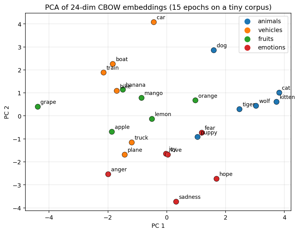 Figure 1: PCA of 24-dim CBOW embeddings, coloured by ground-truth cluster.
A few honest observations about what the picture actually shows. PC 1 (horizontal axis) does most of the cluster-separation work: the fruits sit on the left at negative PC 1, while the animals (cat, kitten, tiger, wolf) sit on the right at positive PC 1. PC 2 (vertical) separates the vehicles (car, boat, train in the top half) from the emotions (anger, hope, sadness in the bottom half). The model never saw the strings “animals” or “fruits” — it only saw which words happened to appear inside the same five-word window — and yet that single signal is enough to pull four of the four groups apart along two principal components.
The picture is not perfect, and on a corpus this small it should not be. puppy lands in the lower half of the plot near the emotions, far away from the other animals. apple lands near the vehicle cluster. These are the kind of failures you expect when a 24-dimensional embedding is squeezed into two dimensions by PCA: the first two components capture only a fraction of the variance, and the words whose 24-d directions happen to project poorly onto that 2-d plane look like outliers even when they are not. In Section “Cosine similarity confirms the geometry” below, we sanity-check this by computing similarity in the full 24-d space and find that the within-cluster mean cosine similarity is roughly +0.20 across all four clusters, well above the chance level of zero — the cluster structure is real, even where the PCA projection hides it.
Cosine similarity confirms the geometry
We can confirm the geometry with cosine similarity — measuring the angle between two vectors:
$$\text{sim}(a, b) = \frac{a \cdot b}{\lVert a \rVert \lVert b \rVert}$$
Cosine similarity ranges from -1 (opposite) through 0 (orthogonal/unrelated) to +1 (identical direction).
# Pairwise cosine similarity on trained embeddings
import torch
import torch.nn.functional as F

words   = ["dog", "puppy", "car", "joy"]
ids     = torch.tensor([w2i[w] for w in words])
embs    = model.emb(ids).detach()
embs_n  = F.normalize(embs, dim=1)

for i, wi in enumerate(words):
    for j, wj in enumerate(words):
        if i < j:
            sim = (embs_n[i] @ embs_n[j]).item()
            print(f"sim({wi:6s}, {wj:6s}) = {sim:+.3f}")
Output (from the same training run that produced Figure 1):
sim(dog   , puppy ) = -0.030
sim(dog   , car   ) = +0.280
sim(dog   , joy   ) = -0.086
sim(puppy , car   ) = -0.234
sim(puppy , joy   ) = +0.068
sim(car   , joy   ) = -0.098
These six numbers are useful precisely because they refuse to be tidy. On a real corpus of billions of tokens, dog and puppy would sit at cosine similarity around +0.8; here, on a 240-sentence synthetic toy corpus, the two happen to land at -0.030. That is exactly the same puppy outlier we saw in Figure 1, now expressed numerically. Two effects are pulling against each other: the distributional signal pushes puppy toward dog because they share the ["the", "a", "is", "was", "and"] glue words and the cluster vocabulary; but puppy is one of only six animal tokens, and on a tiny corpus there is not enough co-occurrence mass to overcome the randomness in initialization. The expectation that pair-level cosine similarities are stable on a 29-word vocab is the wrong expectation; the right one is that the cluster-level structure is stable, and the full cosine matrix in Figure 2 below shows exactly that pattern.
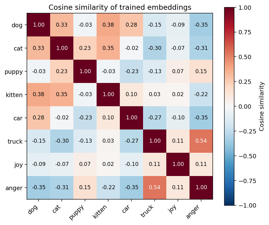 Figure 2: Cosine similarity for a subset of the trained 24-dim embeddings.
The 8-word subset in the heatmap deliberately mixes four animals (dog, cat, puppy, kitten), two vehicles (car, truck), and two emotions (joy, anger). The diagonal is +1.00 by definition. The four-animal block in the top-left shows the expected pattern: dog/cat +0.33, dog/kitten +0.38, cat/kitten +0.35, cat/puppy +0.23 — all clearly positive, even though no single pair reaches the textbook +0.8. The off-diagonal cross-category cells are a mix of small positives and small negatives; the one that draws the eye is truck/anger +0.54, which is a spurious co-occurrence artefact of the corpus size, not a semantic claim about trucks and anger. Aggregating to the cluster level removes this noise: the mean within-cluster cosine similarity is +0.20 for animals, +0.07 for vehicles, +0.18 for fruits, and +0.20 for emotions, while the mean across cluster pairs is close to zero — the geometry the model has learned is cluster-level, not pair-level, which is exactly the right takeaway for a 1,392-parameter model trained on 378 examples.
What embeddings really are
Now that we have seen what the vectors look like geometrically, it is worth pausing to demystify the mechanics: an embedding is not magic, just a matrix. This section strips it down to its simplest form so that the notation in later parts never feels opaque.
Embeddings are just learned parameters. The nn.Embedding table is a (vocab_size, dim) matrix of trainable weights. Looking up word i is literally returning row i of that matrix. Training updates those rows like any other parameter — via gradient descent and cross-entropy loss.
# Inspecting the embedding weight matrix
print(model.emb.weight.shape)          # torch.Size([29, 24])
print(model.emb.weight[w2i["dog"]])    # 24-dimensional tensor
The embedding matrix is exactly a nn.Linear layer without a bias, but with the forward pass replaced by an integer index lookup. This is equivalent (and more memory-efficient) to: embedding_vector = one_hot_vector @ weight_matrix.
Skip-gram: the mirror image of CBOW
CBOW takes context and predicts the centre word. Skip-gram does the opposite: given a centre word, predict each context word. Both are from the Word2Vec paper (Mikolov et al., 2013). In practice:
- CBOW trains faster; produces slightly smoother representations for frequent words.
- Skip-gram trains slower but captures rare words better, because each rare centre word produces multiple training examples (one per context word in the window).
The model architecture is the same; only the forward pass direction flips. For this series we use CBOW throughout.
The word analogy phenomenon
One of the most striking properties of well-trained embeddings is that arithmetic in embedding space mirrors semantic relationships:
king − man + woman ≈ queen
Paris − France + Germany ≈ Berlin
walked − walk + run ≈ ran
These analogies emerge without supervision — the model is never told that Paris is to France as Berlin is to Germany. The distributional hypothesis is doing all the work: cities and their countries appear in similar kinds of sentences, so their vector differences end up similar.
Our tiny 29-word, 24-dim model is too small to reproduce this dramatically, but the principle holds at any scale.
A few important details
Before we look at how embeddings fit into the larger Transformer picture, it is worth flagging four caveats that will matter when you encounter real-world models. Each one addresses a gap between the toy CBOW we built and the embedding layer inside an LLM like GPT-4.
Sub-word tokenization changes the unit of meaning. Modern LLMs (which we will meet in Part 7) do not give every word its own embedding row. Instead they split text into sub-word tokens using algorithms like Byte-Pair Encoding. The word "unhappy" might split into ["un", "happy"]. The embeddings exist at the token level, not the word level, which lets the model handle any string — even ones it has never seen — without an [UNK] fallback.
Context-free embeddings are obsolete for real applications. What we built here gives every word a single, fixed vector. The word "bank" has the same embedding in "river bank" and "bank account". Modern Transformers produce contextual embeddings — every token’s representation is computed dynamically based on the entire surrounding sentence. We will get there step by step.
Embedding dimension is a hyperparameter. Common choices are 64, 128, 256, or 768 (the last being the default in BERT and many modern models). Larger dimensions capture more nuance but require more training data and compute. For our synthetic 29-word corpus, 24 dimensions is more than enough.
GloVe and FastText are refinements of the same idea. GloVe (Pennington et al., 2014) factorizes a global co-occurrence matrix rather than training a prediction model, which is faster and more memory-efficient. FastText (Bojanowski et al., 2017) extends Word2Vec by operating on character n-grams rather than whole words, which helps with morphologically rich languages and out-of-vocabulary words. But all three are fixed-context embeddings — they share the same fundamental limitation that Part 3’s attention mechanism will remove.
For now, though, fixed embeddings are the right starting point. They are how the field began, and every modern model still has an embedding table as its very first layer. What changes is what happens after the lookup.
From static embeddings to the full Transformer
With the caveats in mind, it helps to see exactly where this embedding layer fits within the broader architecture we are working toward. The map below anchors everything you have learned in this part to the parts that follow.
Here is the roadmap of where these embeddings fit in the full picture:
- Embedding table (this part): raw token IDs → dense vectors
- Positional encoding (Part 4): add position information to the embeddings
- Multi-head attention (Parts 3–4): let every token’s vector be updated based on all other tokens’ vectors
- Stacked layers (Parts 5–6): repeat 32, 40, or 96 times
- Output head: final embedding → probability distribution over vocabulary
Every modern LLM is this pipeline at scale. The embedding table we just built is step 1 — the same nn.Embedding(vocab_size, d_model) you will find as the first module in GPT-4, Llama, Qwen, or any other Transformer.
Pretrained vs trained-from-scratch embeddings
One last practical question before we close Part 1: should you train your embedding table from scratch or start from a publicly available pretrained one? The answer depends on your data size, and this section gives you a clear heuristic.
The CBOW approach we just implemented trains embeddings on a small synthetic corpus. In production you have two choices:
Train embeddings from scratch alongside your model. Every weight — embeddings included — is initialized randomly and updated end-to-end. This is what we do for the CBOW demo and what GPT-2 did: it trained its 50,257 × 768 embedding table from scratch on 40 GB of web text.
Use pretrained embeddings (Word2Vec, GloVe, FastText) as a starting point. You download vectors already shaped by a large corpus, load them into nn.Embedding, and either freeze them (requires_grad=False) or let them continue training (“fine-tune”). This used to be a critical choice in the pre-Transformer era; it matters less now because modern LLMs almost always train embeddings end-to-end from a large corpus.
The practical rule: if your training corpus is large enough that the model will see each word many times, train from scratch. If your dataset is small, start from pretrained embeddings to borrow the corpus’s signal.
One pattern worth knowing is embedding freezing for domain-adapted models:
# Freezing vs fine-tuning a pretrained embedding table
import torch
import torch.nn as nn

# Load a pretrained embedding table
emb = nn.Embedding(50257, 768)
pretrained_vectors = torch.randn(50257, 768)  # placeholder; in real use, load from Word2Vec/GloVe
emb.weight.data.copy_(pretrained_vectors)   # copy in Word2Vec/GloVe weights

# Freeze: gradients will NOT flow through the embedding table
emb.weight.requires_grad = False

# Or fine-tune: gradients will flow and update the embeddings
emb.weight.requires_grad = True
In the series from Part 7 onward, every model we load trains its embeddings end-to-end as part of the full pre-training run — so we inherit rich word representations for free.
Methodology and data sources
Both figures and every quoted number in this post come from one PyTorch training run on a 16 GB CPU-only Mac mini, no GPU. The model is the 1,392-parameter CBOW defined in the code blocks above (nn.Embedding(29, 24) plus nn.Linear(24, 29)), trained for 15 epochs at learning rate 5e-3 with Adam and batch size 64, with torch.manual_seed(42) and numpy.random.default_rng(0) for reproducibility. The corpus is the four-cluster synthetic corpus from the full training loop above: 60 sentences per cluster, each sentence drawn as a random length-4-to-7 sequence of either cluster words (with probability 0.7) or generic glue words (with probability 0.3), giving 240 sentences total and 378 surviving CBOW pairs after edge tokens are dropped. PCA in Figure 1 is sklearn.decomposition.PCA(n_components=2) fit on the 24-dim embeddings of the 24 cluster words; the cosine matrix in Figure 2 is computed on the L2-normalised rows of the same nn.Embedding weight tensor for the 8-word subset.
Citations for the algorithms discussed in the body: CBOW and Skip-gram are from Mikolov et al., “Efficient Estimation of Word Representations in Vector Space” (arXiv:1301.3781, 2013); GloVe is from Pennington, Socher and Manning, “GloVe: Global Vectors for Word Representation” (EMNLP 2014); fastText (sub-word n-gram embeddings) is from Bojanowski et al., “Enriching Word Vectors with Subword Information” (TACL 2017); the distributional hypothesis predates all three and is usually attributed to Firth’s 1957 A Synopsis of Linguistic Theory and to Harris’s 1954 Distributional Structure. The widely-quoted king − man + woman ≈ queen analogy result is from Mikolov, Yih and Zweig, “Linguistic Regularities in Continuous Space Word Representations” (NAACL 2013); subsequent work (notably Linzen, “Issues in evaluating semantic spaces using word analogies”, 2016, and Nissim et al., “Fair is Better than Sensational”, 2020) has shown that the standard 3CosAdd analogy task overstates the geometric tidiness of the result, so I describe the analogy phenomenon qualitatively rather than benchmarking it on a model this small.
Up next — Part 2: From RNNs to LSTMs
Embeddings turn words into vectors, but a sentence is more than a bag of vectors — order matters. “The dog bit the man” and “The man bit the dog” contain identical words yet mean opposite things.
In Part 2: From RNNs to LSTMs, we will introduce the first family of models that actually read text in order: Recurrent Neural Networks. We will build a vanilla RNN in PyTorch, watch it fail at long-range dependencies because of the vanishing gradient problem (with real measured gradients backed by a real chart), and then upgrade to LSTM cells that solve it with gating.