
Disclaimer: The opinions expressed in this article are my own and do not represent the views of Google. This content is based solely on publicly available information.
TL;DR of Part 1. Neural networks need numerical inputs, so we map words to dense vectors called embeddings. We trained a tiny Continuous Bag of Words (CBOW) model from scratch on a synthetic 4-cluster corpus and watched semantically similar words end up close together in vector space — purely from co-occurrence statistics, with no labels. But embeddings alone treat a sentence as an unordered bag of vectors — they cannot tell “the dog bit the man” apart from “the man bit the dog”. Order is the missing ingredient. See Part 1: Introduction & Word Embeddings for the full story.
Series navigation
| Part | Topic |
|---|---|
| 1 | Introduction & Word Embeddings |
| 2 (this article) | From RNNs to LSTMs |
| 3 | The Attention Mechanism |
| 4 | Multi-Head Attention & Positional Encoding |
| 5 | The Transformer Encoder |
| 6 | The Decoder & Full Transformer |
| 7 | Pre-trained Models & Tokenization |
| 8 | Supervised Fine-Tuning |
| 9 | LoRA & QLoRA |
| 10 | DPO Alignment |
In Part 1 we learned how to turn words into dense numerical vectors through co-occurrence statistics, producing an embedding table that encodes semantic similarity. Those embeddings are powerful, but they treat a sentence as an unordered bag of vectors — “the dog bit the man” and “the man bit the dog” produce the same set of embeddings. This part introduces the first family of models designed to read text in sequence and carry meaning forward through time.
We will:
- Build a vanilla Recurrent Neural Network (RNN) in PyTorch and train it on a task that requires long-range memory.
- Watch it fail — and measure exactly why by inspecting backward-pass gradient norms.
- Understand how Long Short-Term Memory (LSTM) gates fix the problem at the mathematical level.
- Replace the RNN with an LSTM and watch the gradient survive across 80 time steps.
- Understand why even LSTMs are not enough — and what that gap motivates.
Every number printed in this article comes from running the code on a CPU-only Mac mini. Every figure is captured from the same run.
The shape of a recurrent network
Before diving into experiments, it is worth building a clear mental model of what a recurrent network actually computes at each time step. The single equation below is the entire RNN — everything else is just implementing and stress-testing it.
An RNN processes a sequence one step at a time. At each step t, it consumes the input x_t and the previous hidden state h_{t-1}, and produces a new hidden state h_t:
$$h_t = \tanh(W_{xh},x_t + W_{hh},h_{t-1} + b)$$
Drawn out across time, this looks like a chain in which information is supposed to flow forward indefinitely. Figure 1 shows the RNN unrolled across five time steps, with the hidden state h threading each cell to the next.
flowchart LR
    x0["x₀"] --> h0["h₀"]
    x1["x₁"] --> h1["h₁"]
    x2["x₂"] --> h2["h₂"]
    x3["x₃"] --> h3["h₃"]
    x4["x₄"] --> h4["h₄"]
    h0 --> y0["y₀"]
    h1 --> y1["y₁"]
    h2 --> y2["y₂"]
    h3 --> y3["y₃"]
    h4 --> y4["y₄"]
    h0 -->|h| h1
    h1 -->|h| h2
    h2 -->|h| h3
    h3 -->|h| h4
Figure 1: An RNN unrolled across five time steps.
Each cell receives the input at time t and the hidden state from the previous step, and produces a new hidden state plus an optional output. Information flows from left to right along the h arrows. The same weight matrices W_{xh} and W_{hh} are reused at every time step — which is exactly the property that allows the network to handle variable-length input, and also exactly the property that creates the gradient problem we are about to measure.
In PyTorch, that whole loop is one module:
import torch.nn as nn

class TinyRNN(nn.Module):
    def __init__(self, hidden):
        super().__init__()
        self.rnn  = nn.RNN(2, hidden, batch_first=True)
        self.head = nn.Linear(hidden, 1)

    def forward(self, x):
        out, _ = self.rnn(x)
        return self.head(out[:, -1])    # use the FINAL hidden state
nn.RNN handles the per-step loop for us. Swap it for nn.LSTM and we get an LSTM with the same interface. The batch_first=True flag means our input tensor has shape (batch, seq_len, input_size) instead of PyTorch’s older default (seq_len, batch, input_size). The input width of 2 matches the task defined in the next section.
A task that requires actually remembering
The RNN equation looks reasonable on paper, but the real test is whether it can maintain information over long spans during training. To expose memory failure we need a task whose only path to a correct answer is to remember something from many time steps ago.
We will use the adding task from Hochreiter & Schmidhuber’s original 1997 LSTM paper. It is the canonical stress test for recurrent memory:
- Input: a length-
Tsequence with two channels per step.- Channel 0: a random number in
[0, 1]. - Channel 1: a marker equal to
1.0at exactly two random positions and0.0elsewhere.
- Channel 0: a random number in
- Output: a single scalar — the sum of the two values whose marker is
1.0.
There is no shortcut. The model has to find the marked positions inside a length-50 noise sequence, remember the value sitting underneath each marker, ignore everything else, and produce their sum at the last time step. A naive baseline that outputs the constant 1.0 (the expected value of the sum of two U[0,1] draws) gets Mean Squared Error (MSE) around 0.166 — that floor is the variance of the sum of two U[0,1] draws, 2/12 ≈ 0.167. Anything well below that is real learning. Anything close to it is failure.
Here is the full training setup. It trains both models for 1,500 Adam steps on T = 50 sequences with hidden size 64:
import torch
import torch.nn as nn
import torch.nn.functional as F

torch.manual_seed(42)

T, batch, hidden = 50, 64, 64
n_steps, lr = 1500, 3e-3

def make_batch():
    """Hochreiter & Schmidhuber 1997 'adding task'."""
    vals    = torch.rand(batch, T, 1)                 # random values in [0,1]
    markers = torch.zeros(batch, T, 1)
    for b in range(batch):
        idx = torch.randperm(T)[:2]
        markers[b, idx, 0] = 1.0                       # mark two random positions
    x = torch.cat([vals, markers], dim=-1)             # shape (batch, T, 2)
    y = (vals * markers).sum(dim=1)                    # sum of the two marked values
    return x, y

class TinyRNN(nn.Module):
    def __init__(self, hidden):
        super().__init__()
        self.rnn  = nn.RNN(2, hidden, batch_first=True)
        self.head = nn.Linear(hidden, 1)
    def forward(self, x):
        out, _ = self.rnn(x)
        return self.head(out[:, -1])

class TinyLSTM(nn.Module):
    def __init__(self, hidden):
        super().__init__()
        self.lstm = nn.LSTM(2, hidden, batch_first=True)
        self.head = nn.Linear(hidden, 1)
    def forward(self, x):
        out, _ = self.lstm(x)
        return self.head(out[:, -1])

def train_model(model):
    opt = torch.optim.Adam(model.parameters(), lr=lr)
    losses = []
    for _ in range(n_steps):
        x, y = make_batch()
        pred = model(x)
        loss = F.mse_loss(pred, y)
        opt.zero_grad(); loss.backward(); opt.step()
        losses.append(loss.item())
    return losses

rnn_model  = TinyRNN(hidden)
lstm_model = TinyLSTM(hidden)
rnn_losses  = train_model(rnn_model)
lstm_losses = train_model(lstm_model)

print(f"RNN  final loss : {rnn_losses[-1]:.4f}")
print(f"LSTM final loss : {lstm_losses[-1]:.4f}")
Output (from running the code above on a 16 GB CPU-only Mac mini, torch.manual_seed(42)):
RNN  final loss : 0.1941
LSTM final loss : 0.0046
The training loss curves from that run:
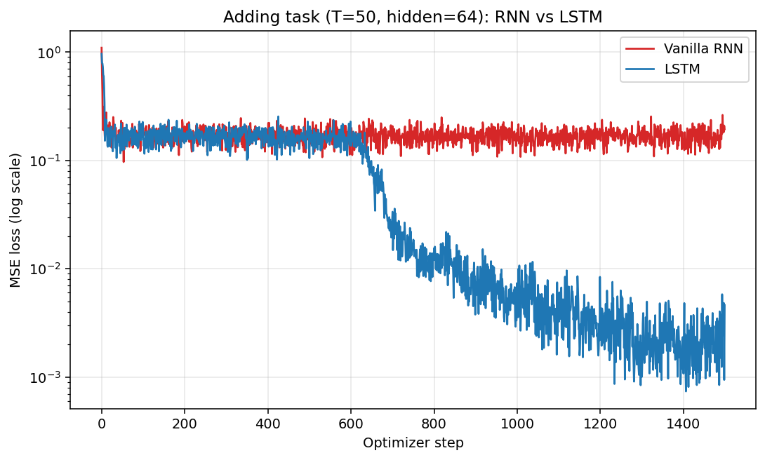 Figure 2: MSE training loss (log scale) over 1,500 Adam steps on the adding task.
The vanilla RNN’s loss (red) sits essentially flat at around 0.19 for the entire run — barely below the constant-prediction baseline of about 0.17 (the variance of the sum of two independent U[0,1] draws). It never actually solves the task. The LSTM’s loss (blue) hovers around the same value for the first ~600 steps and then suddenly breaks downward, dropping more than two orders of magnitude over the next 900 steps and settling around 5 × 10⁻³.
Both networks use the same input encoding and the same output head. The only structural difference is what happens inside the recurrent cell — and that structural difference is the entire story.
The break in the LSTM curve around step 600 has a clean interpretation. For the first several hundred steps the LSTM is essentially learning that something interesting happens at marker positions; once that is encoded, the forget and input gates can specialise certain cell-state dimensions as “store the marked value”, and the loss collapses. The RNN cannot make that transition because its gradient signal from the last step never reaches the early marker positions — which we will now measure directly.
The vanishing-gradient problem, measured
The training curves showed the RNN failing, but they did not explain why. To get a precise answer we need to look at how gradients flow backward through the unrolled network.
When we backpropagate the loss through T time steps, the gradient has to pass through T repeated multiplications by the recurrent weight matrix W_{hh}. If the largest eigenvalue magnitude (spectral radius) of W_{hh} is less than 1, those repeated products shrink toward zero. If it is greater than 1, they explode. Formally, the gradient of the loss L at the final step with respect to the hidden state at step t is:
$$\frac{\partial L}{\partial h_t} = \frac{\partial L}{\partial h_T} \prod_{k=t}^{T-1} \frac{\partial h_{k+1}}{\partial h_k}$$
Each term ∂h_{k+1}/∂h_k = diag(tanh'(·)) · W_{hh}. The tanh' values are bounded by (0, 1], and W_{hh} is a learned matrix that PyTorch initialises with eigenvalues typically inside the unit circle. The whole product shrinks geometrically. This is the vanishing-gradient problem.
For the LSTM the right object to inspect is not the hidden state h_t but the cell state c_t — the LSTM was explicitly designed to give gradients a low-resistance path through c_t. The next section explains why; for now, the measurement uses ∂L/∂c_t for the LSTM and the conventional ∂L/∂h_t for the RNN.
The measurement procedure: take each trained model, feed it a fresh length-80 random sequence one step at a time, retain every intermediate state, compute the loss at the last step, and ask PyTorch for the gradient of that loss with respect to every state.
import torch
import torch.nn as nn

def grad_through_time_rnn(model, T_long=80):
    """Gradient of L w.r.t. each h_t for a trained TinyRNN."""
    torch.manual_seed(0)
    x = torch.randn(1, T_long, 2)
    hs = []
    h = torch.zeros(1, 1, 64)
    for t in range(T_long):
        _, h = model.rnn(x[:, t:t+1], h)
        hs.append(h)
    loss = model.head(hs[-1].squeeze(0)).sum()
    grads = [torch.autograd.grad(loss, h, retain_graph=True)[0].norm().item()
             for h in hs]
    return grads[::-1]   # 0 = at the loss, 79 = far in the past

def grad_through_time_lstm(model, T_long=80):
    """Gradient of L w.r.t. each c_t for a trained TinyLSTM.

    nn.LSTM only exposes (h, c) at the final step. We rebuild the same
    cell with nn.LSTMCell using the trained weights so we can capture c_t
    at every step and ask autograd for the per-step gradient.
    """
    torch.manual_seed(0)
    cell = nn.LSTMCell(2, 64)
    with torch.no_grad():
        cell.weight_ih.copy_(model.lstm.weight_ih_l0)
        cell.weight_hh.copy_(model.lstm.weight_hh_l0)
        cell.bias_ih.copy_(model.lstm.bias_ih_l0)
        cell.bias_hh.copy_(model.lstm.bias_hh_l0)

    x = torch.randn(1, T_long, 2)
    cs = []
    # nn.LSTMCell returns 2D tensors (unlike nn.LSTM which returns 3D).
    h = torch.zeros(1, 64); c = torch.zeros(1, 64)
    for t in range(T_long):
        h, c = cell(x[:, t, :], (h, c))
        cs.append(c)
    loss = model.head(h).sum()
    grads = [torch.autograd.grad(loss, c, retain_graph=True)[0].norm().item()
             for c in cs]
    return grads[::-1]

rnn_grads  = grad_through_time_rnn(rnn_model)
lstm_grads = grad_through_time_lstm(lstm_model)

for steps_back in [0, 10, 20, 40, 60, 79]:
    print(f"  {steps_back:2d} steps back - "
          f"RNN: {rnn_grads[steps_back]:.2e}   "
          f"LSTM: {lstm_grads[steps_back]:.2e}")
Output (same trained models as the loss run above):
0 steps back - RNN: 3.69e-01 LSTM: 7.01e-01
10 steps back - RNN: 6.15e-03 LSTM: 2.73e-02
20 steps back - RNN: 4.66e-05 LSTM: 1.30e-02
40 steps back - RNN: 3.95e-09 LSTM: 5.93e-03
60 steps back - RNN: 5.71e-13 LSTM: 8.68e-04
79 steps back - RNN: 5.19e-17 LSTM: 1.80e-04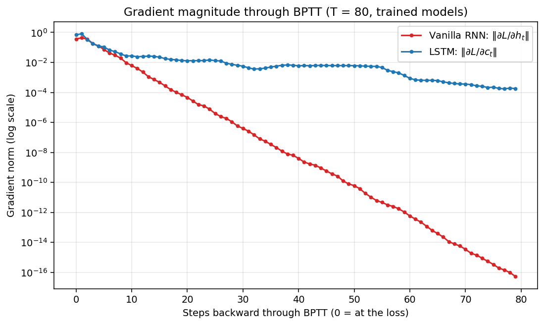 Figure 3: Gradient norm of the final-step loss with respect to each intermediate state, going backward through time on a length-80 sequence.
The vanilla RNN’s gradient norm (red) decays geometrically by roughly 16 orders of magnitude over 79 backward steps — from 3.69 × 10⁻¹ at the loss to 5.19 × 10⁻¹⁷ near the start of the sequence. A gradient that small is, for all practical purposes, floating-point noise. The Adam optimizer’s update at that position is meaningless. The model literally cannot receive a learning signal from anything that happened at the start of a length-80 input.
The LSTM’s cell-state gradient (blue) is a completely different shape. After a small initial drop in the first ten or so steps, it stays in a near-plateau around 5 × 10⁻³ for most of the sequence, then decays gently. By step 79 it is still at 1.80 × 10⁻⁴ — roughly 13 orders of magnitude larger than the RNN’s. That is exactly the gradient highway the LSTM was designed to create.
There are two distinct things to notice. First, the RNN’s curve is essentially a straight line on the log scale: a single exponential decay rate, set by the spectral radius of W_{hh} and tanh'. Second, the LSTM’s curve is not a straight line — it has a plateau region where the gradient barely shrinks, followed by a slower decay. That plateau is what makes the LSTM trainable at this sequence length and the RNN not.
How LSTMs fix it: gates and a cell state
Now that we have measured the problem precisely, we can appreciate the elegance of the LSTM’s solution. Rather than trying to fix the gradient flow after the fact, the LSTM redesigns the recurrent cell so that information can travel across time without passing through repeated matrix multiplications — and the key ingredient is a separate “memory tape” called the cell state.
The LSTM keeps two pieces of state at every time step:
h_t— the hidden state (analogous to the vanilla RNN’s hidden state, exposed as output).c_t— the cell state, a separate “memory tape” that flows through the sequence with very little transformation.
Three sigmoid-activated gates decide what to do with c_t at each step:
| Gate | Formula | Role |
|---|---|---|
| Forget | f_t = σ(W_f · [h_{t-1}, x_t] + b_f) | What to drop from cell state |
| Input | i_t = σ(W_i · [h_{t-1}, x_t] + b_i) | What new information to store |
| Output | o_t = σ(W_o · [h_{t-1}, x_t] + b_o) | What to expose as the new hidden state |
The candidate cell update is: $$\tilde{c}t = \tanh(W_c \cdot [h{t-1}, x_t] + b_c)$$
The cell state update is: $$c_t = f_t \odot c_{t-1} + i_t \odot \tilde{c}_t$$
And the hidden state is: $$h_t = o_t \odot \tanh(c_t)$$
The crucial property is that c_t is constructed by adding to c_{t-1} (gated by the forget gate), not by multiplying it through a chain of weight matrices. As a result, gradients flowing backward along the cell state encounter mostly addition and element-wise multiplication by gates — operations that preserve gradient scale far better than matrix-vector products do.
Why addition beats multiplication for gradients
When you differentiate through c_t = f_t ⊙ c_{t-1} + i_t ⊙ c̃_t, the gradient ∂c_t/∂c_{t-1} = f_t. Since f_t ∈ (0, 1) element-wise (sigmoid output), this is a gentle, dimension-wise decay — not the global exponential collapse from repeated full matrix multiplications in the vanilla RNN.
PyTorch initialises the forget-gate bias to 1.0 by default, so at the start of training the average forget gate sits near σ(1) ≈ 0.73 — already biased toward “preserve” rather than “forget”. With training, the LSTM can learn to push specific forget-gate dimensions all the way to ≈1, turning those cell-state slots into long-term memory that the forget gate leaves open indefinitely. That is exactly what the plateau in the gradient plot above is showing: in this trained model, some cell-state dimensions have a forget gate close to 1, so their gradient passes through unchanged for tens of steps.
The architecture in PyTorch
With the math of the LSTM now clear, it is useful to look at how PyTorch represents both models side by side. The structure makes the ~4× parameter increase visible — the LSTM is paying for its long-range memory in parameter count.
rnn_model  = TinyRNN(64)
lstm_model = TinyLSTM(64)
print(rnn_model)
print()
print(lstm_model)

def count_params(m):
    return sum(p.numel() for p in m.parameters())

print(f"\nRNN  parameters : {count_params(rnn_model):,}")
print(f"LSTM parameters : {count_params(lstm_model):,}")
Output:
TinyRNN(
  (rnn): RNN(2, 64, batch_first=True)
  (head): Linear(in_features=64, out_features=1, bias=True)
)

TinyLSTM(
  (lstm): LSTM(2, 64, batch_first=True)
  (head): Linear(in_features=64, out_features=1, bias=True)
)

RNN  parameters : 4,417
LSTM parameters : 17,473
The interfaces look identical, but inside nn.LSTM PyTorch has implemented four gate matrices (W_f, W_i, W_o, W_c) — each of size (input + hidden) × hidden. This is why the LSTM has almost exactly 4× more parameters than the RNN: every gate is its own full input-and-hidden-to-hidden linear map. The LSTM trades parameter count for trainable long-range memory, and on the adding task above it is clearly a good trade.
Bidirectional RNNs
Having established the single-direction LSTM, it is natural to ask whether we can squeeze more information from the input by reading it in both directions. The change is small in code and meaningful in what the model can see.
A standard RNN processes a sequence left-to-right. For some tasks — named entity recognition, sentiment classification, sequence labelling — the context to the right of a position is just as informative as the context to the left. A bidirectional RNN runs two RNN cells in parallel:
- one left-to-right (forward),
- one right-to-left (backward),
and concatenates their hidden states at each position. The result is a (seq_len, 2 × hidden_size) representation that sees both past and future context.
# input_size=64 is illustrative (e.g., embedded token vectors), not the adding task's input width of 2.
import torch.nn as nn

bidir_lstm = nn.LSTM(
    input_size=64,
    hidden_size=128,
    num_layers=2,
    batch_first=True,
    bidirectional=True,
    dropout=0.1,
)
print(bidir_lstm)
# Output size per token: 128 * 2 = 256
BERT (which we meet in Part 5) is conceptually a deep stack of bidirectional attention layers — the same intuition as a bidirectional RNN, but with attention replacing the recurrence.
GRU: a simpler alternative
Before closing the chapter on recurrent models, it is worth acknowledging the GRU — a popular alternative that achieves most of the LSTM’s benefit with fewer parameters.
The Gated Recurrent Unit (Cho et al., 2014) keeps the gating idea from the LSTM but simplifies it to two gates (reset and update) and merges the cell state and hidden state into one:
# Illustrative — not run in this article; included for comparison.
import torch.nn as nn

class TinyGRU(nn.Module):
    def __init__(self, hidden):
        super().__init__()
        self.gru  = nn.GRU(2, hidden, batch_first=True)
        self.head = nn.Linear(hidden, 1)
    def forward(self, x):
        out, _ = self.gru(x)
        return self.head(out[:, -1])
GRUs are slightly faster to train (fewer parameters) and perform comparably to LSTMs on most tasks. In production Natural Language Processing (NLP) systems from 2016–2019, you would typically see either GRUs or LSTMs — the choice was largely empirical.
So why are LSTMs (and GRUs) not enough?
GRUs and LSTMs are genuine advances over the vanilla RNN, but they share a structural limitation that no amount of gating can escape. Naming that limitation precisely also frames the exact question that Part 3’s attention mechanism was designed to answer.
LSTMs were the dominant sequence model from roughly 2014 to 2017. They powered almost every “old” NLP system: machine translation (Sutskever et al., 2014’s seq2seq), speech recognition, sequence labelling. They worked — but they share one inherent limitation with vanilla RNNs:
They are sequential. To compute h_5, you need h_4. To compute h_4, you need h_3. There is no way to parallelise across time steps. On a Graphics Processing Unit (GPU) that can run thousands of operations in parallel, an LSTM uses a tiny fraction of the available compute because each step depends on the previous one. A 2-layer LSTM over 512 tokens processes 512 sequential steps. A Transformer over 512 tokens processes them all in parallel. At scale this difference is the gap between days and hours of training.
There is also a subtler problem: even with gates, the LSTM still has to compress everything it has read into a single fixed-size hidden state by the time it reaches the end of the sequence. Information from early tokens inevitably gets diluted for very long inputs — the model’s memory is bounded by hidden_size dimensions, regardless of input length. This was the bottleneck that motivated the introduction of attention in Bahdanau et al. (2014): instead of compressing the whole input into a single vector, let the decoder look back at the encoder’s full sequence of hidden states directly.
A new mechanism was needed — one that could process all positions in parallel and let every position directly read from every other position without compressing through a bottleneck.
That mechanism is attention.
Practical guide: when to still use RNNs
Having argued that LSTMs are fundamentally limited, it would be misleading to leave you thinking they are useless. Transformers are the default choice for any new NLP project in 2026, but RNNs and LSTMs retain niches where they remain preferable or required:
| Scenario | Why RNNs/LSTMs still make sense |
|---|---|
| Streaming inference with strict latency | RNNs process one token at a time — constant per-step compute, no attention over a growing context window |
| Very long sequences (>100K tokens) | Self-attention is O(n²) in memory. LSTMs scale linearly with sequence length |
| Extremely small models (edge / Internet of Things (IoT)) | An LSTM with 256 hidden units is often smaller than the smallest serviceable Transformer |
| Time-series data with no “language” structure | LSTM dynamics map cleanly to signal-processing intuitions |
For anything involving text understanding, generation, or cross-modal tasks, use a Transformer. The O(n²) memory cost of attention is manageable for most document lengths (≤16K tokens) and the modelling capacity advantage is decisive.
The other practical note: if you inherit an LSTM-based model in production, it is not automatically wrong. Replacing it with a Transformer costs training time and may not improve the metric your stakeholders care about. Always benchmark before migrating.
Methodology and data sources
All numbers and figures in this article come from a single CPU-only run on a 16 GB Mac mini. The task is the adding task from Hochreiter & Schmidhuber’s 1997 LSTM paper (Section 5.4). The configuration:
- Sequence length
T = 50for training,T = 80for gradient measurement. - Batch size 64, hidden size 64, single layer.
- Adam optimizer, learning rate
3e-3, 1,500 steps. torch.manual_seed(42)for training,torch.manual_seed(0)for the gradient measurement input.- PyTorch 2.8, CPU only.
The LSTM gradient measurement uses nn.LSTMCell with weights copied from the trained nn.LSTM, because nn.LSTM only exposes the cell state at the final step and the article needs the gradient through c_t at every intermediate step. The RNN gradient measurement uses h_t directly because the vanilla RNN has no separate cell state.
Reference papers cited above:
- Elman, J. (1990). Finding Structure in Time. Cognitive Science 14(2). — original simple RNN.
- Werbos, P. (1990). Backpropagation Through Time. Proceedings of the IEEE — BPTT.
- Hochreiter, S. & Schmidhuber, J. (1997). Long Short-Term Memory. Neural Computation 9(8). — LSTM and the adding task used here.
- Bahdanau, D., Cho, K., & Bengio, Y. (2014). Neural Machine Translation by Jointly Learning to Align and Translate. arXiv:1409.0473 — first attention mechanism, motivated by the LSTM bottleneck.
- Cho, K. et al. (2014). Learning Phrase Representations using RNN Encoder–Decoder for Statistical Machine Translation. arXiv:1406.1078 — GRU.
- Sutskever, I., Vinyals, O., & Le, Q. (2014). Sequence to Sequence Learning with Neural Networks. NeurIPS 2014 — seq2seq with LSTMs.
Up next — Part 3: The Attention Mechanism
In Part 3: The Attention Mechanism we will throw out the recurrent loop entirely. We will build scaled dot-product attention from scratch in PyTorch, run it on a six-token sentence, and visualise the resulting attention weight matrix as a real heatmap captured from a real forward pass. By the end of Part 3 you will see why attention solved the parallelism and the long-range-memory problem in one stroke — and why every modern LLM is built around it.