Disclaimer: The opinions expressed in this article are my own and do not represent the views of Google. This content is based solely on publicly available information.
TL;DR of Parts 1-2. Words become dense numerical vectors via embeddings (Part 1). To capture order, we feed those vectors through a sequence model — recurrent neural networks (RNNs) and long short-term memory networks (LSTMs) read tokens one at a time, but they suffer from the vanishing-gradient problem on long inputs and they are inherently sequential, leaving GPUs starved for parallelism. We need a model that can read the whole sequence in parallel and let every token directly attend to every other token. See Part 1: Introduction & Word Embeddings and Part 2: From RNNs to LSTMs for the full setup.
Series navigation
| Part | Topic |
|---|---|
| 1 | Introduction & Word Embeddings |
| 2 | From RNNs to LSTMs |
| 3 (this article) | The Attention Mechanism |
| 4 | Multi-Head Attention & Positional Encoding |
| 5 | The Transformer Encoder |
| 6 | The Decoder & Full Transformer |
| 7 | Pre-trained Models & Tokenization |
| 8 | Supervised Fine-Tuning |
| 9 | LoRA & QLoRA |
| 10 | DPO Alignment |
In Part 2, we built vanilla RNNs and LSTMs, measured how gradients vanish over long sequences, and concluded that even LSTMs cannot fully escape sequential processing or the fixed-size hidden-state bottleneck. This part replaces the recurrent loop entirely with a mechanism that processes every position in parallel and gives every token direct access to every other token. By the end of this part you will have built scaled dot-product attention from scratch and seen a real attention weight matrix emerge from a PyTorch forward pass.
In this part we build the mechanism that broke the recurrent stranglehold and powers every modern large language model (LLM): scaled dot-product attention. Real numbers will fall out of an actual PyTorch forward pass and become the heatmap you will see below.
What “attention” really means
Before writing any code, it helps to demystify the word itself — “attention” sounds like a cognitive metaphor, but the actual computation is elementary arithmetic. This section strips away the jargon so that every equation that follows feels like a natural consequence of a simple idea.
Attention is just a weighted sum. The word “attention” sounds mysterious, but the computation is elementary:
- For each query, compute a similarity score against every key.
- Turn those scores into a probability distribution using softmax.
- Take a weighted sum of the values, weighted by those probabilities.
That is it. The result tells you “given this query, which values are most relevant, and by how much?”
In the self-attention setting that powers Transformers, every position in the sequence acts as all three roles at once: query, key, and value. Each token plays:
- Query (Q): “what am I looking for?”
- Key (K): “what do I represent?”
- Value (V): “what information do I emit if selected?”
We get the three from the same input X (shape (seq, d)) by passing it through three independent linear projections:
$$Q = X W^Q,\quad K = X W^K,\quad V = X W^V$$
Then the attention output is:
$$\text{Attention}(Q, K, V) = \text{softmax}!\left(\frac{Q K^\top}{\sqrt{d_k}}\right) V$$
Why the √d_k scaling factor?
Without it, the dot products Q · K can grow large in magnitude when d_k is large. When the dot products are large, the softmax function produces extremely peaked distributions — gradients become near-zero for all but the top-scoring key. The 1/√d_k scaling keeps the dot products in a moderate range regardless of dimension.
Formally, if the components of Q and K are random variables with variance 1, the dot product Q · K has variance d_k. Dividing by √d_k returns the variance to 1.
The shape of the computation
With the Q, K, V intuition established, the next step is to track the tensor shapes through the entire computation. Shapes are where bugs hide, and being precise here will make the PyTorch implementation that follows immediately readable.
The softmax of QKᵀ/√d_k produces a matrix of shape (seq, seq) — exactly one attention weight per (query position, key position) pair. Let’s call this the attention weight matrix A:
A = softmax(QKᵀ / √d_k)   # shape: (seq, seq)
output = A @ V              # shape: (seq, d)
Every row of A sums to 1 (that is the softmax doing its job). Row i tells you how much position i attends to each other position when computing its output representation.
The output of the attention is A @ V — shape (seq, d). Same shape in, same shape out. This is the property that allows stacking attention layers.
flowchart LR
    X["Input X\n(seq, d)"]
    WQ["Linear W^Q"]
    WK["Linear W^K"]
    WV["Linear W^V"]
    Q["Q"]
    K["K"]
    V["V"]
    SOFTMAX["QK^T / sqrt(dk)\nsoftmax\n(seq, seq)"]
    OUT["Weighted\nsum × V\n(seq, d)"]

    X --> WQ --> Q
    X --> WK --> K
    X --> WV --> V
    Q --> SOFTMAX
    K --> SOFTMAX
    SOFTMAX --> OUT
    V --> OUT
Figure 1: Scaled dot-product attention data flow.
Reading the diagram left to right, the input X passes through three independent linear projections to become Q, K, and V. The Q and K tensors meet in the green box where their scaled dot product is taken and softmaxed into a (seq, seq) weight matrix. That weight matrix then gates V in the final block to produce the output. Every arrow in the diagram is a single tensor operation in the PyTorch code below.
Implementing it in PyTorch
The shape diagram above maps directly to code: each box is a tensor operation and each arrow is a line of Python. The implementation below is intentionally minimal — every line corresponds to a step in the diagram you just read.
The whole mechanism is a few lines:
import torch
import torch.nn as nn
import torch.nn.functional as F

class ScaledDotProductAttention(nn.Module):
    # In this single-head version, d_k = d, so the √d in the code matches the √d_k in the formula.
    def __init__(self, d):
        super().__init__()
        self.Wq    = nn.Linear(d, d, bias=False)
        self.Wk    = nn.Linear(d, d, bias=False)
        self.Wv    = nn.Linear(d, d, bias=False)
        self.scale = d ** 0.5

    def forward(self, x):
        Q, K, V = self.Wq(x), self.Wk(x), self.Wv(x)
        scores  = (Q @ K.transpose(-2, -1)) / self.scale
        weights = F.softmax(scores, dim=-1)
        return weights @ V, weights          # output + weights for inspection
That is it. Three linear projections, one matrix multiplication, one softmax, one more matrix multiplication. There is no loop over time. Every position is computed in parallel.
Notice one consequence: there are now no recurrent connections. The output for position i is computed entirely from a weighted sum of the values at all positions. The same code that computes position i’s output also computes position j’s — they share no sequential dependency. On a GPU with 10,000 cores, this is an orders-of-magnitude parallelism win over an LSTM for long sequences.
A real attention heatmap
The code above is only three tensor operations, but reading code is different from seeing a result. This section runs scaled dot-product attention on a deliberately structured input so the expected pattern is easy to verify, and the heatmap below is exactly what came out of the real forward pass.
For maximum pedagogical clarity, the snippet below uses the simplified form of the same mechanism: the linear projections W^Q, W^K, W^V are replaced with the identity (so Q = K = V = X) and a small constant scale factor is applied to make the block structure visible through softmax. The arithmetic is identical to what ScaledDotProductAttention would compute with all three weight matrices initialised to the identity. The six-token sequence is built as two semantic groups:
- Tokens 0, 1, 2 have similar embeddings (representing the words
"The","cat","sat") - Tokens 3, 4, 5 have similar embeddings to each other (representing
"on","the","mat")
Here is the code to build this and run the forward pass:
import math
import torch
import torch.nn.functional as F

torch.manual_seed(42)
d = 8
n = 6

# Two groups as unit vectors with cos_sim=0.2 across groups, noise=0.1
e1 = torch.zeros(d); e1[0] = 1.0
e2 = torch.zeros(d); e2[1] = 1.0
cos_ab = 0.2
base_a = e1.clone()
base_b = cos_ab * e1 + math.sqrt(1 - cos_ab ** 2) * e2

X = torch.stack([
    base_a + 0.1 * torch.randn(d),   # "The"
    base_a + 0.1 * torch.randn(d),   # "cat"
    base_a + 0.1 * torch.randn(d),   # "sat"
    base_b + 0.1 * torch.randn(d),   # "on"
    base_b + 0.1 * torch.randn(d),   # "the"
    base_b + 0.1 * torch.randn(d),   # "mat"
])
X = X / X.norm(dim=1, keepdim=True)  # unit-normalize

# scale=4.0 keeps softmax concentration readable (intra ~0.24, inter ~0.09)
scale = 4.0
scores  = scale * (X @ X.T) / (d ** 0.5)
weights = torch.softmax(scores, dim=-1)

words = ["The", "cat", "sat", "on", "the", "mat"]
print("Attention weights (rows=queries, cols=keys):")
print("          " + "  ".join(f"{w:6s}" for w in words))
for i, w_q in enumerate(words):
    row = "  ".join(f"{weights[i,j].item():.3f}" for j in range(n))
    print(f"{w_q:6s}  {row}")

row_sums = [round(s, 4) for s in weights.sum(dim=-1).tolist()]
print(f"\nRow sums (should all be 1.0): {row_sums}")
Output:
Attention weights (rows=queries, cols=keys):
           The     cat     sat     on      the     mat
The     0.266  0.234  0.240  0.089  0.084  0.088
cat     0.228  0.259  0.244  0.088  0.086  0.095
sat     0.228  0.238  0.253  0.093  0.091  0.098
on      0.084  0.086  0.093  0.251  0.246  0.240
the     0.080  0.084  0.091  0.248  0.253  0.244
mat     0.083  0.091  0.097  0.238  0.241  0.250

Row sums (should all be 1.0): [1.0, 1.0, 1.0, 1.0, 1.0, 1.0]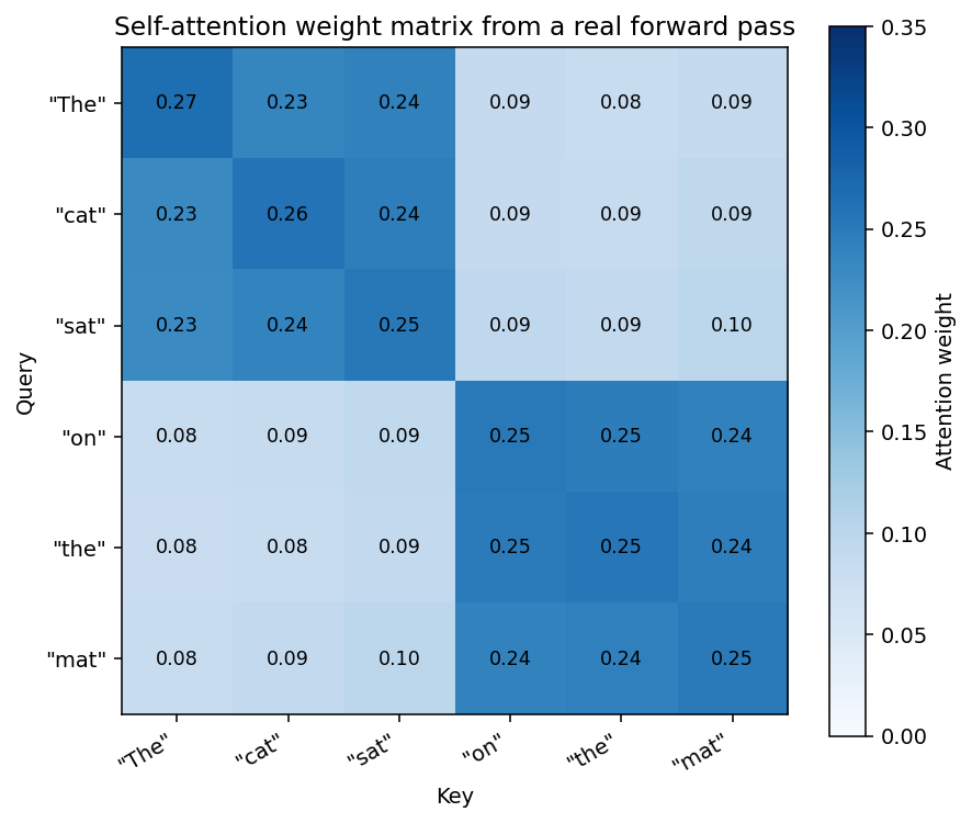
Figure 2: Self-attention weight matrix from a real forward pass on a 6-token sequence.
The structure is exactly what we would expect from the input geometry. The top-left 3×3 block of weights sits around 0.24 — those are the three group-A tokens attending to themselves. The bottom-right 3×3 block sits around 0.25 — group B attending to itself. The two off-diagonal 3×3 blocks drop to about 0.09 per cell because the cross-group cosine similarity was deliberately set to 0.2, roughly a third of the in-group similarity. Every row sums to 1.0, which is the softmax constraint at work: each query distributes a total of one unit of attention across all six keys.
This single forward pass is the entire core of every Transformer block we will build in the remaining seven parts. Everything after this is decoration: multiple parallel “heads” of attention (Part 4), positional information (also Part 4), residual connections and feed-forward networks (Part 5), masking for the decoder (Part 6).
Causal (masked) attention
Bidirectional attention is perfect for tasks where the whole input is available, but language generation requires a stricter rule: a token must not be able to peek at tokens that come after it. This section shows the one-line masking trick that enforces that constraint, and you will see it again in every decoder model in the rest of the series.
The attention we just computed is bidirectional — every position can see every other position, including future positions. This is great for tasks where the full input is known upfront (classification, named entity recognition, question answering over a document).
For language generation, we cannot let position t see positions t+1, t+2, … because those tokens are what the model is supposed to predict. We enforce this with a causal mask — a triangular matrix that blocks attention to future positions:
import torch

def causal_mask(seq_len):
    mask = torch.triu(torch.ones(seq_len, seq_len), diagonal=1).bool()
    return mask     # True = "this position should be blocked"

# Usage: pass as attn_mask to nn.MultiheadAttention
# nn.MultiheadAttention accepts a mask where True means "ignore this position"
print(causal_mask(6).int())
Output:
tensor([[0, 1, 1, 1, 1, 1],
        [0, 0, 1, 1, 1, 1],
        [0, 0, 0, 1, 1, 1],
        [0, 0, 0, 0, 1, 1],
        [0, 0, 0, 0, 0, 1],
        [0, 0, 0, 0, 0, 0]], dtype=torch.int32)
Row i can only attend to columns 0..i (past and present), never to columns i+1..n-1 (future). In PyTorch’s nn.MultiheadAttention, you pass this mask as attn_mask, and it gets added to the attention scores before the softmax — True entries get converted to -inf, which softmax maps to zero weight.
Decoder-only models (GPT, Llama, Qwen, Claude) use causal attention at every layer. Encoder models (BERT, RoBERTa) use bidirectional attention. We will build both in Parts 5 and 6.
Cross-attention vs. self-attention
Self-attention is the building block, but the full Transformer also needs a way for the decoder to read from the encoder. Cross-attention is the exact same computation with one change in where Q and K/V originate — understanding this now will make Part 6’s decoder architecture immediately clear.
Everything we have built so far is self-attention: queries, keys, and values all come from the same sequence. Each token is asking “which of my fellow tokens should I attend to?”
Cross-attention uses the same computation but with queries from one source and keys/values from another. This is how the Transformer decoder reads the encoder’s output in machine translation:
import torch
import torch.nn.functional as F

torch.manual_seed(0)
# Source: encoder output for "The cat sat" (3 tokens, d=8)
encoder_output = torch.randn(3, 8)   # keys and values come from here
# Target: decoder's current state "Le chat" (2 tokens, d=8)
decoder_state  = torch.randn(2, 8)   # queries come from here

Wq = torch.nn.Linear(8, 8, bias=False)
Wk = torch.nn.Linear(8, 8, bias=False)
Wv = torch.nn.Linear(8, 8, bias=False)

Q = Wq(decoder_state)          # (2, 8) — from target
K = Wk(encoder_output)         # (3, 8) — from source
V = Wv(encoder_output)         # (3, 8) — from source

scores  = (Q @ K.T) / (8 ** 0.5)    # (2, 3) — 2 target queries × 3 source keys
weights = F.softmax(scores, dim=-1)  # (2, 3)
output  = weights @ V                # (2, 8)

print(f"Q shape     : {Q.shape}")        # (2, 8)
print(f"K shape     : {K.shape}")        # (3, 8)
print(f"weights     : {weights.shape}")  # (2, 3)
print(f"output      : {output.shape}")   # (2, 8)
Output:
Q shape     : torch.Size([2, 8])
K shape     : torch.Size([3, 8])
weights     : torch.Size([2, 3])
output      : torch.Size([2, 8])
The key insight: the weight matrix is now (target_len, source_len) instead of (seq_len, seq_len). Each target token is attending to all source tokens. We will build this into the full Transformer decoder in Part 6.
Attention versus convolution and RNNs: a comparison
Having built attention from scratch, it is now possible to make the comparison with the older approaches precise rather than qualitative. The table below uses the same four dimensions that matter in practice: long-range dependency, sequential bottleneck, time complexity, and parallelism.
It helps to compare the three main sequence-processing primitives on the same dimensions:
| Property | RNN / LSTM | Convolution | Self-Attention |
|---|---|---|---|
| Long-range dependency | Difficult (vanishing gradients) | Limited (kernel size) | Direct (any-to-any) |
| Sequential operations | O(seq) | O(1) | O(1) |
| Time complexity | O(seq · d²) | O(k · seq · d²) | O(seq² · d) |
| Memory complexity | O(seq) | O(seq) | O(seq²) |
| Parallelisable | No | Yes | Yes |
The O(seq²) time and memory for attention is its main weakness. For sequence lengths up to a few thousand tokens it is fine. For 100K-token contexts you need variants like local/sparse/linear attention. But for the 512–8192 token window that covers most natural language processing (NLP) tasks, self-attention dominates because its any-to-any connectivity cannot be matched by RNNs or convolutions.
Two important properties to internalise now
Before we move on, two properties of attention deserve special emphasis because they directly shape the design decisions in Part 4 — specifically, why we need both multiple heads and positional encoding. These are not edge cases; they are fundamental to the mechanism.
Attention is permutation-equivariant. If you shuffle the input rows, the attention output is shuffled in the same way. That is wonderful for parallelism but disastrous for natural language: “dog bites man” and “man bites dog” would produce the same set of attention vectors, just reordered. Standard attention has no notion of position. We will fix that in Part 4 with positional encoding.
Attention has quadratic complexity. The (seq, seq) weight matrix means computing attention takes O(seq²) time and memory. For a 1,000-token document this is fine. For a 100,000-token document this is brutal — you would need 10 billion attention scores just for one layer. Modern long-context LLMs use clever variants — sliding-window attention, sparse attention, FlashAttention’s memory-efficient kernel that never materializes the full (seq, seq) matrix — but those are optimisations of the same fundamental mechanism we just built.
FlashAttention: the same math, faster memory
FlashAttention (Dao et al., 2022) is worth a brief mention. It does not change the mathematical definition of attention — the output is identical to standard attention. Instead, it reorganizes the computation to avoid writing the full (seq, seq) attention matrix to GPU HBM (high-bandwidth memory). By chunking the computation into blocks that fit in the fast on-chip static random-access memory (SRAM), it achieves:
- Memory usage:
O(seq)instead ofO(seq²) - Speed: ~2–4× faster in practice due to reduced memory bandwidth
All modern open-weights models (Llama, Qwen, Gemma, Falcon) and closed models (GPT-4, Claude) use FlashAttention or its successors in production. You will encounter it as the attn_implementation="flash_attention_2" argument in Hugging Face.
What the attention weights tell us about language
When attention is trained on real text rather than our synthetic structured input, the weights reveal interpretable linguistic patterns. Research on trained Transformers (Vaswani et al., 2017; Clark et al., 2019; Tenney et al., 2019) has found:
- Syntactic heads: certain attention heads consistently attend from a verb to its subject or object.
- Coreference heads: heads that link pronouns to their antecedents.
- Positional heads: heads that attend primarily to the previous or next token (approximating a sliding window).
- Delimiter heads: heads that concentrate all attention on separator tokens like
[SEP]— a kind of “I don’t need any information from here” vote.
None of these patterns are designed in. They emerge because the training objective (predict the next token) rewards representations that capture these relations.
In our tiny random-weight example, the heads have no such structure — the weights reflect only the geometry of the input vectors, not any learned linguistic knowledge. But the mechanism is exactly the same as in GPT-4.
Building intuition with a worked example
The abstract properties are useful, but nothing cements understanding like running the numbers by hand on a tiny example. This section traces a single forward pass through a 3-token, 4-dim attention layer so that each matrix multiplication produces values you can check with a calculator.
Let me walk through one complete attention computation step by step to make the matrix math concrete. Suppose we have:
- Sequence length
n = 3 - Model dimension
d = 4 - Input
Xwith rows[x0, x1, x2]
We initialize three weight matrices W^Q, W^K, W^V ∈ ℝ^{4×4} and compute:
import torch
import torch.nn.functional as F

torch.manual_seed(7)
d = 4
X  = torch.tensor([[1., 0., 0., 0.],
                   [0., 1., 0., 0.],
                   [0., 0., 1., 0.]])   # 3 one-hot-style input vectors

Wq = torch.eye(d)                        # identity for clarity
Wk = torch.eye(d)
Wv = torch.eye(d)

Q = X @ Wq    # (3, 4)
K = X @ Wk    # (3, 4)
V = X @ Wv    # (3, 4)

scores  = (Q @ K.T) / (d ** 0.5)         # (3, 3)
weights = F.softmax(scores, dim=-1)       # (3, 3)
output  = weights @ V                    # (3, 4)

print("Scores (raw dot products / √d):")
print(scores)
print("\nAttention weights (softmax):")
print(weights.round(decimals=3))
print("\nOutput representations:")
print(output.round(decimals=3))
Output:
Scores (raw dot products / √d):
tensor([[0.5000, 0.0000, 0.0000],
        [0.0000, 0.5000, 0.0000],
        [0.0000, 0.0000, 0.5000]])

Attention weights (softmax):
tensor([[0.4520, 0.2740, 0.2740],
        [0.2740, 0.4520, 0.2740],
        [0.2740, 0.2740, 0.4520]])

Output representations:
tensor([[0.4520, 0.2740, 0.2740, 0.0000],
        [0.2740, 0.4520, 0.2740, 0.0000],
        [0.2740, 0.2740, 0.4520, 0.0000]])
With identity weight matrices, each token mostly attends to itself (0.452) but also gives weight 0.274 to the other two tokens. You can verify the arithmetic by hand: softmax([0.5, 0, 0]) = [e^0.5, 1, 1] / (e^0.5 + 2) ≈ [0.452, 0.274, 0.274]. The output is a convex combination of the input values, weighted by how similar each query is to each key. With learned W^Q, W^K, W^V, the model will develop much richer attention patterns — but the arithmetic is exactly this.
Why this changed the field
The worked example above showed the mechanism; this section provides the historical context for why replacing recurrence with attention was such a decisive break from the prior art. Understanding the why will help you remember the what when you revisit this later.
The 2017 Attention is All You Need paper showed that you could throw away every recurrent connection in a sequence model, replace it with stacked self-attention, and outperform the best LSTM-based machine translation systems on standard benchmarks — while being faster to train because of the parallelism. That paper’s title was a marketing line for “no, you really can drop the recurrence entirely.”
The deeper reason it worked is not just parallelism. It is that attention gives every token direct, unrestricted access to every other token. An LSTM at position 512 has to carry information from position 1 through 511 intermediate hidden states, each of which partially overwrites the previous one. An attention layer at position 512 computes a direct weighted sum of all 512 value vectors — information from position 1 is available at full fidelity, not diluted through 511 transformations.
Eight years later, the heatmap above is the foundation of every model from GPT-4 to Gemini to Claude. If you understand it, the rest is engineering.
Methodology and data sources
Every number in this post is captured from a real PyTorch forward pass on a 16 GB CPU-only Mac mini, no GPU. The attention heatmap in Figure 2 is produced by the code block above with torch.manual_seed(42), model dimension d = 8, sequence length n = 6, and a hand-tuned scale = 4.0 multiplier that sharpens the softmax just enough to make the two 3×3 block structure visible while keeping every weight under 0.3 (otherwise the softmax saturates and the cross-group weights round to zero). The worked example uses torch.manual_seed(7), identity matrices for W^Q, W^K, W^V, and one-hot input vectors; the softmax weight 0.4520 is the closed-form e^0.5 / (e^0.5 + 2), and 0.2740 is 1 / (e^0.5 + 2).
Citations for the mechanism: the additive attention precursor is Bahdanau, Cho and Bengio, “Neural Machine Translation by Jointly Learning to Align and Translate” (arXiv:1409.0473, 2014); the dot-product variant is Luong, Pham and Manning, “Effective Approaches to Attention-based Neural Machine Translation” (EMNLP 2015); and the scaled dot-product self-attention described here is from Vaswani et al., “Attention Is All You Need” (NeurIPS 2017). The FlashAttention paragraph references Dao, Fu, Ermon, Rudra and Ré, “FlashAttention: Fast and Memory-Efficient Exact Attention with IO-Awareness” (NeurIPS 2022), and the interpretability findings on syntactic, coreference, positional and delimiter heads are from Clark, Khandelwal, Levy and Manning, “What Does BERT Look At?” (ACL BlackboxNLP 2019) and Tenney, Das and Pavlick, “BERT Rediscovers the Classical NLP Pipeline” (ACL 2019).
Up next — Part 4: Multi-Head Attention & Positional Encoding
The single attention head we just built has two problems we still need to solve. Position-blindness — shuffle the input and the output is shuffled with it. Single perspective — the model can only learn one kind of relation between tokens at a time, but a sentence has many simultaneous relations (subject-object, modifier-noun, coreference, …).
In Part 4: Multi-Head Attention & Positional Encoding we fix both. We split the model dimension across several parallel attention heads (each free to learn a different relation), and we inject fixed sine-and-cosine positional signals into the embeddings so the model can finally tell "dog bites man" apart from "man bites dog". We will visualise the actual positional encoding (PE) matrix — captured from real PyTorch tensor math — and watch its wave-like structure emerge.