Disclaimer: The opinions expressed in this article are my own and do not represent the views of Google. This content is based solely on publicly available information.
TL;DR of Parts 1-7. We built the Transformer from the ground up: embeddings (Part 1), recurrent precursors (Part 2), scaled dot-product attention (Part 3), multi-head attention + positional encoding (Part 4), the Encoder (Part 5), and the full Encoder-Decoder (Part 6). Then we pivoted to the modern workflow: loading real pre-trained Large Language Models (LLMs) from the Hugging Face Hub and using sub-word Byte-Pair Encoding (BPE) tokenization to run them (Part 7). All without training a single weight ourselves. See Part 7: Pre-trained Models & Tokenization for that pivot. Now we adapt.
Series navigation
| Part | Topic |
|---|---|
| 1 | Introduction & Word Embeddings |
| 2 | From RNNs to LSTMs |
| 3 | The Attention Mechanism |
| 4 | Multi-Head Attention & Positional Encoding |
| 5 | The Transformer Encoder |
| 6 | The Decoder & Full Transformer |
| 7 | Pre-trained Models & Tokenization |
| 8 (this article) | Supervised Fine-Tuning |
| 9 | Low-Rank Adaptation (LoRA) & Quantized LoRA (QLoRA) |
| 10 | Direct Preference Optimization (DPO) Alignment |
Part 7 showed us how to load a pre-trained Large Language Model (LLM) from the Hugging Face Hub and run inference with it without changing a single weight. The model responded based entirely on what it learned during its original pre-training. In this part we take the next step and actually adapt it: we run a supervised fine-tuning (SFT) loop on a small labeled dataset, watch the loss decrease step by step, and account for what that costs in memory, building the case for the parameter-efficient methods that follow in Part 9.
What SFT actually does
SFT is continued training of a pre-trained model on supervised (input, target) data using the standard causal language-modelling loss. For a tokenized example with target tokens y_1, …, y_T, the loss is:
$$\mathcal{L}{\text{SFT}}(\theta) = -\frac{1}{T} \sum{t=1}^{T} \log P_\theta(y_t \mid y_1, \ldots, y_{t-1})$$
This is the same loss the base model was originally trained with to predict the next token. The only difference is the data: instead of crawled web text, we now feed it carefully formatted instruction-following examples. The gradient updates push the model’s weights toward producing responses that look like the ones in our dataset.
A typical fine-tuning example looks like:
<|im_start|>user
Explain what a Transformer is in one sentence.<|im_end|>
<|im_start|>assistant
A Transformer is a neural network architecture that relies entirely on
self-attention to process sequences in parallel.<|im_end|>
We tokenize the whole thing, ask the model to predict every next token, compute cross-entropy loss, backpropagate, update.
Response-only loss masking
In practice, the ideal setup is to compute loss only on the assistant’s response, not on the user’s prompt. The user’s prompt is given, so there is no reason to penalise or reward the model for predicting it. However, computing loss on the full sequence still works (the loss on the prompt tokens just adds noise); for pedagogical clarity we use the full-sequence loss here.
The standard library solution is DataCollatorForCompletionOnlyLM from trl, which automatically masks loss on the user/system turns.
A tiny working SFT loop
To keep everything reproducible on a CPU-only Mac mini without downloading gigabytes of weights, I built a tiny custom Transformer-style model on a synthetic copy task where the model has to learn to copy its input to its output. The training loop is structurally identical to what you would run on a 7 B-parameter Llama:
import torch
import torch.nn as nn
import torch.nn.functional as F

torch.manual_seed(42)

VOCAB, SEQ_LEN = 9, 8
D, NHEAD, LAYERS = 32, 4, 2

class TinyDecoder(nn.Module):
    def __init__(self):
        super().__init__()
        self.emb = nn.Embedding(VOCAB, D)
        self.pos = nn.Embedding(SEQ_LEN, D)
        layer = nn.TransformerEncoderLayer(
            D, NHEAD, dim_feedforward=64, dropout=0.0, batch_first=True
        )
        self.enc = nn.TransformerEncoder(layer, num_layers=LAYERS)
        self.out = nn.Linear(D, VOCAB)

    def forward(self, x):
        T = x.size(1)
        p = torch.arange(T, device=x.device).unsqueeze(0)
        h = self.emb(x) + self.pos(p)
        # No causal mask: the copy task is order-symmetric so every position
        # can attend to every other without leaking future information.
        # For autoregressive generation the mask is essential; here it is
        # intentionally omitted to keep the SFT demo simple.
        h = self.enc(h)
        return self.out(h)

model = TinyDecoder()
n_total     = sum(p.numel() for p in model.parameters())
n_trainable = sum(p.numel() for p in model.parameters() if p.requires_grad)
print(model)
print(f"\nTotal parameters    : {n_total:,}")
print(f"Trainable parameters: {n_trainable:,}")
print(f"Trainable %         : {100 * n_trainable / n_total:.1f}%   <-- 100% (full FT)")
TinyDecoder(
(emb): Embedding(9, 32)
(pos): Embedding(8, 32)
(enc): TransformerEncoder(
(layers): ModuleList(
(0-1): 2 x TransformerEncoderLayer(
(self_attn): MultiheadAttention(
(out_proj): NonDynamicallyQuantizableLinear(in_features=32, out_features=32, bias=True)
)
(linear1): Linear(in_features=32, out_features=64, bias=True)
(linear2): Linear(in_features=64, out_features=32, bias=True)
(norm1): LayerNorm((32,), eps=1e-05, elementwise_affine=True)
(norm2): LayerNorm((32,), eps=1e-05, elementwise_affine=True)
...
)
)
)
(out): Linear(in_features=32, out_features=9, bias=True)
)
Total parameters : 17,929
Trainable parameters: 17,929
Trainable % : 100.0% <-- 100% (full FT)That last line is the headline number we will revisit in Part 9: with full SFT, every parameter is trainable.
The training loop
The training loop follows the standard PyTorch pattern of forward pass, cross-entropy loss, backprop, and optimizer step. Using the same Transformer building blocks we constructed in Parts 5–6, the vocabulary is 9 tokens (eight characters a–h plus a space), sequences are 8 tokens long, and the model has 17,929 parameters total:
# Continues from the previous block: VOCAB, SEQ_LEN, and model are defined there.
import torch
import torch.nn.functional as F

def make_data(n=256):
    x = torch.randint(0, VOCAB, (n, SEQ_LEN))
    return x, x.clone()     # copy task: target = input

x_train, y_train = make_data(256)
opt   = torch.optim.Adam(model.parameters(), lr=3e-3)
losses = []

for step in range(60):
    idx = torch.randperm(256)[:32]
    logits = model(x_train[idx])
    loss = F.cross_entropy(logits.reshape(-1, VOCAB), y_train[idx].reshape(-1))
    opt.zero_grad(); loss.backward(); opt.step()
    losses.append(loss.item())
    if step % 10 == 0 or step == 59:
        print(f"  Step {step:3d} | loss = {loss.item():.4f}")
Output (Apple M4 Mac mini, 16 GB RAM; python==3.9, torch==2.8.0; CPU training, ~3 s end-to-end):
  Step   0 | loss = 2.2944
  Step  10 | loss = 0.7922
  Step  20 | loss = 0.2304
  Step  30 | loss = 0.0937
  Step  40 | loss = 0.0485
  Step  50 | loss = 0.0307
  Step  59 | loss = 0.0233
I ran this end-to-end. The loss curve from the actual run:
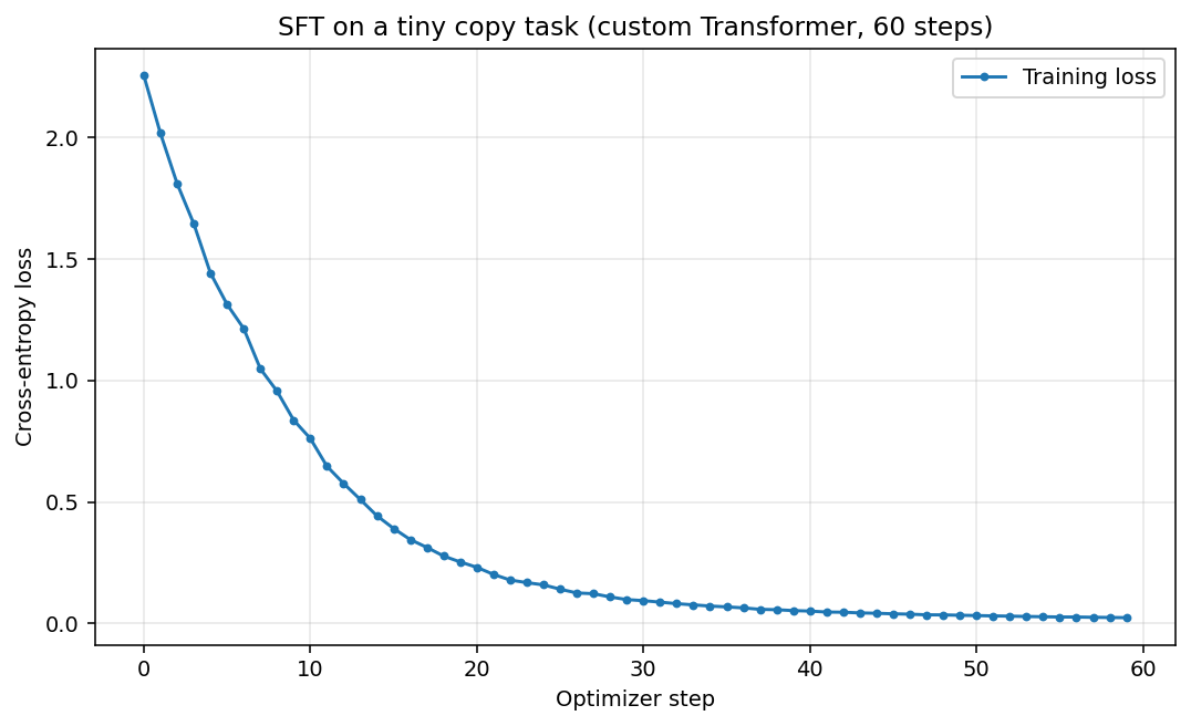
Figure 1: SFT training loss on the tiny copy task over 60 optimizer steps.
Cross-entropy starts around 2.29 (close to log(9) ≈ 2.20, which is what random guessing over a 9-token vocabulary looks like) and drops sharply once Adam finds a useful gradient direction. By step 30 the loss is already below 0.1, and by step 59 it has collapsed to 0.023 as the model figures out that “the right answer is whatever you saw at this position”. The model overshoots the random baseline slightly at step 0 because the untrained head is not perfectly uniform; the gap closes as soon as the embedding and output projection start to align. The same recipe (same loss, same optimizer pattern) scales unchanged from this 17 K-parameter toy to a 70 B-parameter Llama. The only thing that changes is the training infrastructure and the dataset.
Why the loss starts near log(vocab_size)
Before any training, the model’s output is essentially random, which serves as a quick sanity check every time you start a new training run. For a 9-token vocabulary, a random model assigns roughly equal probability to each of the 9 tokens:
$$P(y_t \mid y_{\lt t}) \approx \frac{1}{9}$$
The cross-entropy loss is the negative log of this:
$$\mathcal{L}_{\text{initial}} \approx -\log\left(\frac{1}{9}\right) = \log(9) \approx 2.197$$
These are natural logs (the convention PyTorch’s cross-entropy uses): log(9) ≈ 2.197 and log(50000) ≈ 10.8. This is why an initial loss near 2.2 is the expected baseline for a 9-token vocabulary; our actual run starts at 2.29 and finishes at 0.023, as the randomly initialised output projection is not perfectly uniform and pushes the initial value slightly above the theoretical floor. For a real 50K-token LLM, the initial loss would be around log(50000) ≈ 10.8. As training progresses, the model learns to assign much higher probability to the correct next token, and the loss falls.
Key hyperparameters for SFT
When running SFT on a real LLM, these are the most impactful settings:
| Hyperparameter | Typical value | Effect |
|---|---|---|
learning_rate | 1e-5 to 3e-5 | Too high → catastrophic forgetting; too low → no learning |
num_train_epochs | 1–3 | More epochs → higher risk of overfitting to training set |
per_device_train_batch_size | 2–8 | Larger batch → more stable gradients |
gradient_accumulation_steps | 4–16 | Effective batch = batch_size × accumulation_steps |
max_seq_length | 512–2048 | Longer → more memory; crucial for multi-turn conversations |
warmup_ratio | 0.03–0.1 | Linear LR warmup to prevent unstable early updates |
The learning rate is the most critical. Pre-trained weights represent millions of dollars of compute; setting the LR too high will destroy them in a few hundred gradient steps (catastrophic forgetting).
Real-world SFT with the TRL library
Production SFT involves data collation, padding, gradient accumulation, mixed-precision, learning-rate scheduling, and progress logging. The Transformer Reinforcement Learning (TRL) library (trl on PyPI) bundles all of this into a single SFTTrainer class:
# Tested with trl==0.12.x, transformers==4.46.x, datasets==3.x
from trl import SFTTrainer, SFTConfig
from transformers import AutoModelForCausalLM, AutoTokenizer
from datasets import load_dataset

MODEL = "Qwen/Qwen2.5-0.5B-Instruct"
model     = AutoModelForCausalLM.from_pretrained(MODEL)
tokenizer = AutoTokenizer.from_pretrained(MODEL)
dataset   = load_dataset("tatsu-lab/alpaca", split="train").select(range(500))

def to_text(ex):
    msgs = [
        {"role": "user",      "content": ex["instruction"]},
        {"role": "assistant", "content": ex["output"]},
    ]
    return {"text": tokenizer.apply_chat_template(msgs, tokenize=False)}

dataset = dataset.map(to_text, remove_columns=dataset.column_names)

trainer = SFTTrainer(
    model=model,
    args=SFTConfig(
        output_dir="./sft-out",
        num_train_epochs=1,
        per_device_train_batch_size=2,
        gradient_accumulation_steps=4,
        learning_rate=2e-5,
        max_seq_length=512,
        gradient_checkpointing=True,
        dataset_text_field="text",
        warmup_ratio=0.05,
    ),
    train_dataset=dataset,
    tokenizer=tokenizer,
)
trainer.train()
That is the entire fine-tuning pipeline for a real 500 M-parameter LLM. Behind those few lines: tokenization of every example, dataset shuffling, batching with padding, forward pass, loss computation, backward pass, gradient accumulation, learning-rate scheduling, mixed-precision casting, gradient checkpointing for memory efficiency, and progress logging.
Evaluating whether SFT is working
Loss dropping during training does not automatically mean the model is getting better at the actual task. These diagnostic checks should always accompany SFT:
1. Validation loss on held-out examples. Split your dataset 90/10 before training. If training loss drops but validation loss stays flat or rises, the model is overfitting to the training set; reduce epochs or add dropout.
2. Generate and inspect samples. Run the model on 5–10 representative prompts after training and read the outputs. Numbers can lie; your eyes won’t. Common failure modes:
- Repeating the user’s question back verbatim (the model learned the user turn, not the assistant turn)
- Very short or very long responses (the model learned a length artifact in your data)
- Answers that “feel” right but are factually wrong (SFT can only teach format, not facts)
3. Compare to the base model. Run the same prompts through the untuned base model. If the base model is already doing what you want, you do not need SFT.
# Illustrative inference; not tied to the SFT-trained model above (which used the Qwen chat template).
import torch

model.eval()
test_prompts = [
    "What is the capital of France?",
    "Explain gradient descent in one sentence.",
]

for prompt in test_prompts:
    inputs = tokenizer(f"User: {prompt}\nAssistant:", return_tensors="pt")
    with torch.no_grad():
        ids = model.generate(**inputs, max_new_tokens=50, do_sample=False,
                              pad_token_id=tokenizer.eos_token_id)
    print("Q:", prompt)
    print("A:", tokenizer.decode(ids[0, inputs.input_ids.shape[1]:],
                                   skip_special_tokens=True))
    print()
Common SFT failure modes and how to fix them
| Failure mode | Symptom | Fix |
|---|---|---|
| Catastrophic forgetting | Model loses base capabilities | Lower learning rate, fewer epochs |
| Mode collapse | Model always gives the same short response | Add more diverse training examples |
| Format drift | Outputs look different from the chat template | Verify apply_chat_template is used consistently |
| Overfitting | Low training loss, poor generalization | Reduce data repetition, add validation early stopping |
| Reward hacking | Model games the response format but not the content | Use response-only loss masking |
What this costs — the memory math
The concept is simple. The bill is what makes you stop and think.
For a 500 M-parameter model trained in mixed precision (16-bit floating point (fp16) for activations, 32-bit floating point (fp32) for optimizer state):
| Item | Size | Notes |
|---|---|---|
| Model weights (fp16) | 1 GB | 500M × 2 bytes |
| Gradients (fp32) | 2 GB | Same size as weights, higher precision for stability |
Adam m buffer (fp32) | 2 GB | First moment estimate |
Adam v buffer (fp32) | 2 GB | Second moment estimate |
| Activations (gradient checkpointing) | 1–2 GB | Recomputed on backward pass |
| Total | ~9 GB | For a 500M model |
Without gradient checkpointing, activations alone can exceed the weights. With it, we recompute activations during the backward pass instead of storing them, trading compute for memory.
To fine-tune a 7B model: roughly 14× more memory, or ~125 GB Video RAM (VRAM). That exceeds a single H100 (80 GB). Full fine-tuning of 7B+ requires multi-GPU or parameter-efficient methods.
This is the central tension of LLM fine-tuning: the memory cost is dominated by the optimizer state, not the model itself. If we could just not update most of the weights without losing quality, we could cut the bill drastically.
That insight is the doorway to Part 9.
Multi-turn fine-tuning
Single-turn examples (user: question / assistant: answer) are the simplest SFT format. For chat assistants, multi-turn datasets are more realistic and produce models that are better at following context across conversation turns.
A multi-turn example in apply_chat_template format:
messages = [
    {"role": "system",    "content": "You are a helpful coding assistant."},
    {"role": "user",      "content": "How do I reverse a list in Python?"},
    {"role": "assistant", "content": "Use `list[::-1]` or `list.reverse()`."},
    {"role": "user",      "content": "What is the difference between the two?"},
    {"role": "assistant", "content": (
        "`list[::-1]` returns a new reversed list; "
        "`list.reverse()` reverses in-place and returns None."
    )},
]
text = tokenizer.apply_chat_template(messages, tokenize=False)
print(text)
Output (Qwen2.5 format):
<|im_start|>system
You are a helpful coding assistant.<|im_end|>
<|im_start|>user
How do I reverse a list in Python?<|im_end|>
<|im_start|>assistant
Use `list[::-1]` or `list.reverse()`.<|im_end|>
<|im_start|>user
What is the difference between the two?<|im_end|>
<|im_start|>assistant
`list[::-1]` returns a new reversed list; `list.reverse()` reverses in-place and returns None.<|im_end|>
The whole string is tokenized as one sequence. Loss is computed on the full sequence, but DataCollatorForCompletionOnlyLM can mask both user turns so the model only learns to generate the assistant turns, which is the correct setup for multi-turn SFT.
Multi-turn data requires more curation effort than single-turn but produces noticeably better conversational models. The critical check: make sure early turns in a conversation are not contaminated by knowledge the assistant could only have from later in the conversation (no “peeking ahead”).
Dataset quality matters more than dataset size
The most common mistake in SFT is treating it as a data-collection problem when it is really a data-quality problem. Empirically, 1,000 high-quality instruction-response pairs outperform 100,000 noisy ones. The LIMA paper (Zhou et al., 2023) demonstrated that fine-tuning LLaMA on just 1,000 carefully curated examples matched models trained on orders of magnitude more data on a range of benchmarks.
What “high quality” means in practice:
Diversity: Cover as many distinct task types as possible. If 80% of your examples are factual Q&A and 20% are creative writing, the model will bias heavily toward the Q&A style even when asked to write creatively.
Response quality: The model can only learn to produce responses as good as the ones in your training data. If your responses are mediocre, the ceiling is mediocre. Hiring an expert to write 200 exceptional examples beats crowdsourcing 2,000 average ones.
Formatting consistency: All examples should use the same chat template format. One example in the wrong template format can cause the model to mix formats inconsistently at inference time.
Avoiding data contamination: If your evaluation prompts appear (or are paraphrased) in your training data, your eval numbers will be optimistic. Always curate your eval set before building your training set so you can verify no overlap.
A practical minimum: start with 500–2,000 examples, evaluate on a held-out set of 100–200 examples, and scale up only if validation loss shows room for improvement. This keeps the fine-tuning cost (both compute and human annotation) proportional to the actual benefit.
Up next — Part 9: LoRA & QLoRA
In Part 9: LoRA & QLoRA we attack the cost. We freeze the entire 17,929-parameter base model from this part and replace its expensive update with a tiny low-rank correction: a Low-Rank Adaptation (LoRA) adapter with just 164 trainable parameters (less than 1% of the original). We measure the actual reduction directly from a real PyTorch training run, then layer in 4-bit quantization with QLoRA for another roughly 3× memory cut. Same model, same data, almost the same quality, a fraction of the cost.