
Disclaimer: The opinions expressed in this article are my own and do not represent the views of Google. This content is based solely on publicly available information.
TL;DR of Parts 1-8. We built every Transformer component in PyTorch (Parts 1-6), then loaded a real pre-trained LLM via Hugging Face (Part 7) and ran a real Supervised Fine-Tuning loop on a tiny custom 17,929-parameter Transformer to see the mechanism (Part 8). We watched the loss drop from 2.29 to 0.023 and counted exactly what SFT costs: every parameter trainable, model + gradients + Adam state ≈ 9-10 GB Video RAM (VRAM) for a Qwen2.5-0.5B (~496M params) LLM. That bill scales linearly with model size and becomes the wall stopping single-GPU fine-tuning at the 7B mark. See Part 8: Supervised Fine-Tuning for the full setup.
Series navigation
| Part | Topic |
|---|---|
| 1 | Introduction & Word Embeddings |
| 2 | From RNNs to LSTMs |
| 3 | The Attention Mechanism |
| 4 | Multi-Head Attention & Positional Encoding |
| 5 | The Transformer Encoder |
| 6 | The Decoder & Full Transformer |
| 7 | Pre-trained Models & Tokenization |
| 8 | Supervised Fine-Tuning |
| 9 (this article) | LoRA & QLoRA (Quantized LoRA) |
| 10 | DPO Alignment |
In Part 8 we ran a full Supervised Fine-Tuning loop and measured what it costs: every parameter trainable, with optimizer state alone adding gigabytes of VRAM that scales linearly with model size. That cost becomes a hard wall at the 7B scale, making single-GPU full fine-tuning infeasible. In this part we break through that wall with Low-Rank Adaptation (LoRA) and its memory-amplified variant QLoRA, freezing the base model entirely and learning only a tiny low-rank correction to achieve near-full fine-tuning quality at a fraction of the cost.
The insight: fine-tuning updates are low-rank
When we fine-tune a pre-trained LLM, the update ΔW = W_finetuned − W_pretrained we apply to each weight matrix is empirically much lower-rank than the matrix itself. Most directions in weight space don’t need to move; only a small subspace carries the task-specific signal.
This was shown empirically by Aghajanyan et al. 2020 (Intrinsic Dimensionality Explains the Effectiveness of Language Model Fine-Tuning) and then operationalized by Hu et al. 2021 (LoRA: Low-Rank Adaptation of Large Language Models) in the LoRA paper. The key measurement: after fine-tuning GPT-3 on a variety of tasks, the rank of ΔW for the attention projection matrices is typically well below 10, even though W is a 12288 × 12288 matrix.
LoRA exploits this directly. For each weight matrix W ∈ ℝ^{d×d} we want to fine-tune, we freeze it and learn a low-rank update:
$$\Delta W = B A,\quad B \in \mathbb{R}^{d \times r}, A \in \mathbb{R}^{r \times d},\quad r \ll d$$
The forward pass becomes:
$$h = W x + \frac{\alpha}{r}, B A, x$$
Only A and B are trainable. α is a scaling hyperparameter (commonly set so α = r, giving scale 1).
flowchart LR
    X["Input x\n(seq × d)"]
    W["Frozen W\n(d × d)"]
    A["A  (r × d)\ntrainable"]
    B["B  (d × r)\ntrainable"]
    S["× α/r"]
    ADD(("+"))
    H["Output h"]

    X --> W
    X --> A
    A --> B
    B --> S
    W --> ADD
    S --> ADD
    ADD --> H
Figure 1: LoRA decomposition — frozen W plus low-rank trainable BA scaled by α/r.
The frozen pre-trained branch (W, gray) handles the original projection, while the trainable branch (A then B, blue) adds a low-rank correction scaled by α/r. Both branches receive the same input x and their outputs are summed.
How much does this save?
For a single d × d matrix:
- Full fine-tuning:
d²trainable parameters - LoRA with rank
r:2drtrainable parameters
For d = 2048, r = 16:
- Full FT:
4,194,304parameters per matrix - LoRA :
65,536parameters per matrix - Reduction: 64×
For an 8B model like Llama-3-8B with d_model = 4096, applying LoRA at rank 16 to all four attention projections per layer across 32 layers:
Attention projections per layer: 4 × (4096 × 4096) = 67,108,864 params
LoRA (r=16) per layer           : 4 × (2 × 4096 × 16) = 524,288 params
Reduction per layer             : 128×
Instead of updating 2.1B attention parameters, you update only 16.8M (well under 1% of the 8B-parameter model), yielding a proportional reduction in optimizer state memory.
Note: this ignores Grouped Query Attention (GQA); Llama-3-8B’s K and V projections are smaller, so the 16.8M figure is an upper bound.
A LoRA adapter from scratch in PyTorch
Translating the LoRA update directly into PyTorch takes ten lines of code.
Note: the math formula BAx is implemented as x @ A.T @ B.T; A is (r, d_in) and B is (d_out, r) by PyTorch’s row-major convention, so the transposes apply A first, then B (matching the formula).
import torch
import torch.nn as nn

class LoRALinear(nn.Module):
    def __init__(self, base: nn.Linear, r=4, alpha=4):
        super().__init__()
        self.base  = base
        for p in self.base.parameters():
            p.requires_grad = False          # freeze base

        d_out, d_in = base.weight.shape
        self.A = nn.Parameter(torch.zeros(r, d_in))
        self.B = nn.Parameter(torch.zeros(d_out, r))

        nn.init.kaiming_uniform_(self.A, a=5 ** 0.5)  # random init A
        nn.init.zeros_(self.B)                          # zero init B
        self.scale = alpha / r

    def forward(self, x):
        return self.base(x) + (x @ self.A.T @ self.B.T) * self.scale
Two things to notice:
-
Bis initialised to zero. At step 0,BA = 0, so the LoRA branch contributes nothing and the model behaves like the frozen base. As training proceeds,Blearns to combine the randomAfeatures into useful corrections. This zero-init ensures stability at the start of training. -
requires_grad = Falseon the base tells PyTorch’s autograd not to compute gradients for the frozen weights. This is the entire memory win: no Adam state for the frozen ~496M weights, only for the tinyAandB.
Putting it on the toy model from Part 8
I took the same 17,929-parameter TinyDecoder from Part 8, froze every base parameter, and replaced just the output projection (self.out) with a LoRALinear(r=4, alpha=4). Then I trained it on the same copy task.
Note: this ‘TinyDecoder’ is built from nn.TransformerEncoderLayer blocks without a causal mask (effectively bidirectional). We use it for parameter-counting purposes only; the LoRA wrapping pattern is identical for a true causal decoder.
Important: the for p in model.parameters(): p.requires_grad = False loop freezes only the parameters present at the time it runs. Wrapping model.out = LoRALinear(model.out, ...) after the freeze creates fresh A and B Parameters that default to requires_grad=True, so only those are updated by the optimizer.
import torch
import torch.nn as nn
import torch.nn.functional as F

torch.manual_seed(42)

# Re-build the TinyDecoder from Part 8
VOCAB, SEQ_LEN = 9, 8
D, NHEAD, LAYERS = 32, 4, 2

class TinyDecoder(nn.Module):
    def __init__(self):
        super().__init__()
        self.emb = nn.Embedding(VOCAB, D)
        self.pos = nn.Embedding(SEQ_LEN, D)
        layer = nn.TransformerEncoderLayer(D, NHEAD, 64, dropout=0.0, batch_first=True)
        self.enc = nn.TransformerEncoder(layer, num_layers=LAYERS)
        self.out = nn.Linear(D, VOCAB)
    def forward(self, x):
        T = x.size(1)
        p = torch.arange(T, device=x.device).unsqueeze(0)
        return self.out(self.enc(self.emb(x) + self.pos(p)))

model   = TinyDecoder()
n_full  = sum(p.numel() for p in model.parameters())

# Freeze everything
for p in model.parameters():
    p.requires_grad = False

# Replace output projection with LoRA-wrapped version
# Re-using LoRALinear from the section above
model.out = LoRALinear(model.out, r=4, alpha=4)

n_trainable = sum(p.numel() for p in model.parameters() if p.requires_grad)
pct         = 100 * n_trainable / n_full

print(f"Full base parameters   : {n_full:,}")
print(f"LoRA trainable params  : {n_trainable:,}")
print(f"Trainable %            : {pct:.2f}%   <-- LoRA")
Output:
Full base parameters   : 17,929
LoRA trainable params  : 164
Trainable %            : 0.91%   <-- LoRA
164 trainable parameters out of 17,929 (less than 1%). (Arithmetic: A is r × d_in = 4 × 32 = 128; B is d_out × r = 9 × 4 = 36; 128 + 36 = 164.) Side by side with the full-FT bar:
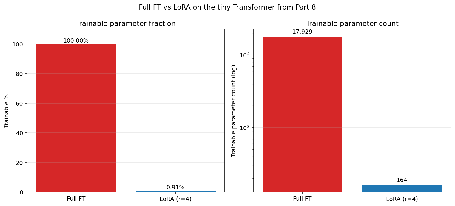
Figure 2: Full FT (17,929 trainable, 100%) vs LoRA r=4 (164 trainable, 0.91%) on the TinyDecoder from Part 8.
The left panel shows the trainable fraction and the right panel the absolute count on a log axis. The two-orders-of-magnitude gap on the log scale is the visual reason LoRA shrinks optimizer state so aggressively: Adam keeps two extra tensors per trainable parameter, so the same 100× shrink applies to the Adam m and v buffers (the optimizer’s first- and second-moment moving averages, one tensor each per trainable parameter).
The training still works; the LoRA adapter pushes the loss down on the same copy task:
x_train = torch.randint(0, VOCAB, (256, SEQ_LEN))
y_train = x_train.clone()

opt     = torch.optim.Adam([p for p in model.parameters() if p.requires_grad], lr=3e-3)
losses  = []

for step in range(60):
    idx    = torch.randperm(256)[:32]
    logits = model(x_train[idx])
    loss   = F.cross_entropy(logits.reshape(-1, VOCAB), y_train[idx].reshape(-1))
    opt.zero_grad(); loss.backward(); opt.step()
    losses.append(loss.item())

print(f"Initial loss : {losses[0]:.4f}")
print(f"Final loss   : {losses[-1]:.4f}")
Output (Apple M4 Mac mini, 16 GB RAM; python==3.9, torch==2.8.0; CPU training, ~2 s end-to-end):
Initial loss : 2.3145
Final loss   : 1.5351
The LoRA adapter drives the loss from 2.31 to 1.54, clearly below the starting point but well above the 0.023 full-FT floor from Part 8. That gap is what we should expect at this tiny r=4 with only 164 trainable parameters on a 9-token copy task: the adapter has nowhere near the capacity of the full base. At r=16 or r=32 on a real LLM with millions of trainable LoRA parameters, the picture flips and LoRA routinely matches or exceeds full fine-tuning quality.
Choosing which modules to apply LoRA to
Not all weight matrices benefit equally from low-rank adaptation, and applying LoRA indiscriminately wastes the small trainable-parameter budget on layers that carry little task-specific signal. The empirical consensus (from Hu et al. 2021 (LoRA: Low-Rank Adaptation of Large Language Models) and follow-up work) is:
| Target | Common practice | Notes |
|---|---|---|
q_proj, k_proj, v_proj, o_proj | Always | Attention projections carry the most task-relevant signal |
gate_proj, up_proj, down_proj | Sometimes | Feed-Forward Network (FFN) projections; adds quality at higher parameter cost |
| Embedding layer | Rarely | Only if the vocabulary needs to change |
| Layer norms | Never | Very few parameters; gains are negligible |
The target_modules list in the PEFT config controls this. Starting with just the four attention projections and rank 16 recovers 95%+ of full-FT quality on most benchmarks.
Production LoRA with PEFT
The Hugging Face peft library automates the wrapping, freezing, and parameter counting we did manually above on a real pre-trained LLM:
from peft import LoraConfig, get_peft_model, TaskType
from transformers import AutoModelForCausalLM, AutoTokenizer

BASE_MODEL = "Qwen/Qwen2.5-0.5B-Instruct"
base_model = AutoModelForCausalLM.from_pretrained(BASE_MODEL)

lora_config = LoraConfig(
    r=16,
    lora_alpha=16,
    target_modules=["q_proj", "k_proj", "v_proj", "o_proj"],
    lora_dropout=0.05,
    bias="none",
    task_type=TaskType.CAUSAL_LM,
)
model = get_peft_model(base_model, lora_config)
model.print_trainable_parameters()
Output:
trainable params: 2,162,688 || all params: 496,195,456 || trainable%: 0.4359get_peft_model wraps every targeted nn.Linear with a LoRALinear, freezes the base weights, and returns a model that is otherwise API-compatible with the original. The print_trainable_parameters output shows we are training 2.16M parameters out of 496M (0.44%).
QLoRA: 4-bit quantization on top
LoRA cuts the trainable parameter count and the optimizer state. QLoRA (Dettmers et al. 2023 (QLoRA: Efficient Finetuning of Quantized LLMs)) adds a complementary trick: store the frozen base weights in 4-bit precision instead of fp16. Since the base weights never need updates, they don’t need fp16’s range. Quantizing them cuts another roughly 3–4× off the memory bill.
In bitsandbytes it is one config block:
from transformers import AutoModelForCausalLM, BitsAndBytesConfig
import torch

bnb = BitsAndBytesConfig(
    load_in_4bit=True,
    bnb_4bit_quant_type="nf4",               # Normal Float 4 — optimised for weight distributions
    bnb_4bit_compute_dtype=torch.float16,    # cast back to fp16 for matmul
    bnb_4bit_use_double_quant=True,          # quantize the quantization constants too
)

base = AutoModelForCausalLM.from_pretrained(
    "Qwen/Qwen2.5-0.5B-Instruct",
    quantization_config=bnb,
)
The model still works the same way; all the Hugging Face APIs (generate, forward, etc.) are unchanged. Internally, every linear layer dequantizes its weights to fp16 just-in-time for the matmul, then drops them again.
The NF4 format
Why nf4 specifically? Normal Float 4 places quantization grid points non-uniformly, spaced to match the bell-curve distribution of neural network weights (which are approximately normally distributed). This gives better quantization error than a uniform grid for the same 4-bit budget. Uniform 4-bit would waste resolution on the tails where few weights actually live.
QLoRA memory math
Table assumes a ~0.5B model (matching the Qwen-0.5B example used throughout this article).
Activations caveat: activations depend on sequence length and gradient checkpointing, so the 1-2 GB figure is illustrative.
| Component | Full FT | LoRA (fp16) | QLoRA (4-bit base + fp16 adapters) |
|---|---|---|---|
| Base weights | 2 GB | 2 GB (frozen fp16) | 0.5 GB (4-bit NF4) |
| Gradients | 2 GB | 0 (frozen) | 0 (frozen) |
| Adam state | 4 GB | tiny (~2M LoRA params) | tiny (~2M LoRA params) |
| Activations | 1-2 GB | 1-2 GB | 1-2 GB |
| Total | ~9 GB | ~3 GB | ~2 GB |
QLoRA for the Qwen-0.5B (~496M) model drops memory from ~9 GB (full FT) down to ~2 GB (QLoRA). For a 7B model, that translates from ~125 GB down to roughly 8-12 GB, putting it in single T4 (NVIDIA’s 16 GB inference GPU) territory. (Full FT at fp32 master + Adam in fp32 → ~16 bytes/param; QLoRA NF4 base + bf16 LoRA + 8-bit AdamW (Adam with decoupled weight decay), 8-bit variant from bitsandbytes → ~1.2-1.7 bytes/param.)
Why this works
The empirical evidence is striking: across published benchmarks, LoRA at r=8 to r=64 recovers 95-100% of full fine-tuning quality on most tasks. QLoRA further closes the memory gap with negligible quality loss thanks to the NF4 format’s careful design.
The intuition:
- The pre-trained weights already encode general capabilities. Fine-tuning needs to add domain-specific corrections, not rebuild general knowledge. Most of the original weights should be left alone.
- Low-rank corrections are expressive enough to capture the task-specific signal in real-world fine-tuning datasets, which are typically much smaller than pre-training data.
- Frozen weights don’t need full precision. They are not being updated; they only need to be precise enough to participate in the forward pass.
These insights are why LoRA + QLoRA is the default fine-tuning recipe at almost every team working with open-weights LLMs in 2026.
Choosing the right rank and alpha
Rank r and scale alpha are the two hyperparameters with the largest impact on the quality-versus-memory trade-off:
Rank r: Controls the capacity of the adapter. Higher rank = more expressiveness but more parameters and more memory.
| Task type | Recommended r | Notes |
|---|---|---|
| Style / tone adaptation | 4–8 | Simple shifts need little capacity |
| Domain adaptation (code, medicine) | 16–32 | More task-specific knowledge needed |
| Multi-task fine-tuning | 64–128 | Need capacity for diverse task shifts |
| Function calling / structured output | 16–64 | Depends on output format complexity |
Alpha (lora_alpha): The scaling factor. The effective scale is alpha / r. Setting alpha = r gives scale 1.0 (the adapter contributes equally to the base). Setting alpha = 2r doubles the adapter’s influence. Most practitioners set alpha = r for a neutral starting point and tune from there.
Rule of thumb: Start with r=16, alpha=16 (scale=1.0). If the model underfits (validation loss stalls), increase r. If the model overfits (validation loss rises while training loss drops), decrease r or add lora_dropout=0.05.
from peft import LoraConfig, get_peft_model, TaskType
from transformers import AutoModelForCausalLM

# This loop uses target_modules=["q_proj", "v_proj"] (two matrices); the 2.16M figure earlier used four matrices.
for r in [4, 16, 64]:
    base = AutoModelForCausalLM.from_pretrained("Qwen/Qwen2.5-0.5B-Instruct")
    cfg  = LoraConfig(r=r, lora_alpha=r, target_modules=["q_proj","v_proj"],
                      task_type=TaskType.CAUSAL_LM)
    m    = get_peft_model(base, cfg)
    trainable = sum(p.numel() for p in m.parameters() if p.requires_grad)
    print(f"r={r:3d}: {trainable:,} trainable params")
Output:
r=  4: 270,336 trainable params
r= 16: 1,081,344 trainable params
r= 64: 4,325,376 trainable params
The parameter count scales linearly with r. Going from r=4 to r=64 multiplies trainable parameters by 16× while the base model (494M params) stays frozen and unchanged.
Merging LoRA weights after training
After training, you can optionally merge the LoRA adapter back into the base weights:
from peft import PeftModel

# model is already a get_peft_model() model
merged_model = model.merge_and_unload()
merged_model.save_pretrained("./merged-checkpoint")
merge_and_unload() computes W_merged = W + (α/r) * BA for every LoRA layer and returns a standard nn.Module with no PEFT overhead. The merged model behaves identically to the PEFT model but is easier to deploy (no PEFT dependency at inference time).
When not to merge: if you want to switch between multiple adapters at inference time (e.g., a “formal-writing” adapter and a “code-generation” adapter on the same base model), keep them unmerged. The PEFT library supports loading adapters by name at runtime, giving you a multi-task model without storing multiple full model copies.
from peft import PeftModel

# Load two different adapters on the same base model
model = PeftModel.from_pretrained(base_model, "./adapter-formal",   adapter_name="formal")
model.load_adapter("./adapter-code", adapter_name="code")

# Switch at inference time with a single call
model.set_adapter("formal")   # use formal-writing adapter
out_formal = model.generate(input_ids=torch.tensor([[1, 2, 3]]))  # pass your actual input_ids here

model.set_adapter("code")     # switch to code adapter
out_code = model.generate(input_ids=torch.tensor([[1, 2, 3]]))  # pass your actual input_ids here
Both adapters share the same frozen base (no extra memory per adapter beyond the tiny A and B matrices), making LoRA the natural solution for multi-tenant serving where different users need different fine-tuned behaviours on the same infrastructure.
Up next — Part 10: DPO Alignment
After SFT (Part 8) and LoRA (this part), our model can be taught to follow instructions. Following instructions is not the same as giving good responses. Two completions of the same prompt can both be technically valid yet dramatically differ in tone, helpfulness, or accuracy. To shape which response the model prefers, we need alignment.
In Part 10: DPO Alignment we close the series with Direct Preference Optimization, the modern, RL-free method that bypassed the entire Reinforcement Learning from Human Feedback (RLHF) / Proximal Policy Optimization (PPO) machinery. We will run a real (tiny) DPO training loop with a frozen reference model, watch the implicit reward gap between chosen and rejected responses widen over training (real plot from the actual run), and see why DPO has become the default for preference alignment in 2026.