Disclaimer: The opinions expressed in this article are my own and do not represent the views of Google. This content is based solely on publicly available information.
TL;DR of Parts 1-9. We built every piece of a Transformer from scratch in PyTorch (Parts 1-6), then loaded a real pre-trained LLM (Part 7) and ran first a full Supervised Fine-Tuning (SFT) loop (Part 8) and then a parameter-efficient LoRA loop (Part 9), watching the trainable-parameter count drop from 100% to 0.91% of the same model with comparable quality. SFT and LoRA teach a model what to say. They cannot teach it which of several valid responses to prefer. That last gap is what alignment closes. See Part 9: LoRA & QLoRA for the technique we will build on top of.
This article is Part 10 of the series. The DPO derivation and code below are self-contained; familiarity with SFT (Part 8) and LoRA (Part 9) helps but is not required.
Series navigation
| Part | Topic |
|---|---|
| 1 | Introduction & Word Embeddings |
| 2 | From RNNs to LSTMs |
| 3 | The Attention Mechanism |
| 4 | Multi-Head Attention & Positional Encoding |
| 5 | The Transformer Encoder |
| 6 | The Decoder & Full Transformer |
| 7 | Pre-trained Models & Tokenization |
| 8 | Supervised Fine-Tuning |
| 9 | LoRA & QLoRA |
| 10 (this article) | DPO Alignment |
In Part 9 we shrank the trainable-parameter count from 100% down to under 1% using LoRA and QLoRA, making it possible to fine-tune a 7B model on a single GPU. Efficient fine-tuning only teaches a model what to say; it still cannot tell the model which of several valid responses to prefer when different answers differ in tone, helpfulness, or safety. That last gap is what alignment closes, and in this final part we will implement Direct Preference Optimization (DPO), the modern RL-free method that has replaced the classical PPO/RLHF pipeline as the alignment default.
This is the final part of the series. We close the loop with Direct Preference Optimization (DPO), the RL-free alignment technique that has displaced the classical PPO/RLHF pipeline as the default as of 2026. We will:
- Understand why alignment is its own problem distinct from SFT.
- Walk through the brief history of PPO/RLHF and why DPO replaced it.
- Derive the DPO loss and implement it directly in PyTorch.
- Run a tiny DPO training loop and watch the implicit reward gap widen, captured from a real run.
Two valid answers, only one preferred
Imagine asking a model “Explain the Transformer architecture in simple terms.” Two responses are both technically correct:
Response A: “The Transformer uses self-attention to process all tokens in parallel.”
Response B: “Yes okay so the Transformer it has these things called attention heads that look at all the other tokens at the same time which is good because Recurrent Neural Networks (RNNs) were slow and so basically that means the model can be parallelized which is faster and also more accurate I think.”
Both convey the same factual content. SFT (which we did in Part 8) cannot distinguish them; it would happily train on either as a valid (prompt, response) pair. To make the model prefer A over B, we need a different training signal: comparisons, not single ground-truth answers.
The general framing is preference data: a triple (prompt, y_chosen, y_rejected) where a human (or another LLM) has decided that y_chosen is the better response. Modern preference datasets like argilla/Capybara-Preferences or Anthropic/hh-rlhf consist of millions of such triples.
Why alignment needs its own training stage
SFT teaches the model to produce outputs that look like the examples in the training set. Because the examples in a typical SFT dataset were collected by the same team that built the model, they are not necessarily a complete representation of what users actually want.
Alignment via preference feedback adds a second signal: not just “does this output look like a training example” but “does the model rank outputs the way humans do?” These two objectives pull in slightly different directions:
- SFT: minimize cross-entropy on training text → model learns to imitate the training set distribution
- Alignment: maximise the likelihood of chosen-over-rejected → model learns user preferences
Both are needed. A model that skipped SFT and only did alignment would have no formatting or instruction-following baseline to work from. A model that skipped alignment would follow a format but not necessarily be helpful or harmless.
The classical answer: PPO/RLHF
The 2022 InstructGPT paper from OpenAI introduced the canonical Reinforcement Learning from Human Feedback recipe, which is a three-stage pipeline:
- SFT the base model on demonstrations (Part 8).
- Train a separate reward model: a small network that maps
(prompt, response)to a scalar reward, fit on the preference data so it scores chosen responses higher than rejected ones. - Run PPO (Proximal Policy Optimization, a reinforcement-learning algorithm) where the policy model generates responses, the reward model scores them, and PPO uses gradient ascent on those rewards to update the policy, with a Kullback–Leibler (KL) divergence penalty to keep the policy close to the original SFT model.
Classical PPO/RLHF pipeline:
flowchart LR
    A["Stage 1\nSFT"] --> B["Stage 2\nReward Model"]
    B --> C["Stage 3\nPPO\n(policy + ref + RM)"]
Modern DPO pipeline:
flowchart LR
    A["Stage 1\nSFT"] --> B["Stage 2 — DPO\n(single classification loss\non preference pairs)"]
Figure 1: Classical PPO/RLHF (top) vs DPO (bottom). Classical PPO/RLHF requires three stages (SFT, reward-model training, PPO loop with three model copies; RM = reward model). DPO collapses stages 2 and 3 into a single offline classification loss.
Stage 3 is where the engineering pain lives. PPO requires:
- Three model copies in memory (policy, frozen reference, reward model).
- On-policy rollouts at every training step, where the policy generates fresh samples sequentially (one token at a time).
- A KL penalty coefficient that must be carefully tuned to prevent the policy from drifting too far from the reference and collapsing.
This is doable but expensive and finicky. The InstructGPT team needed serious engineering to make it work at scale.
The DPO insight
The 2023 DPO paper (Rafailov et al., Direct Preference Optimization: Your Language Model is Secretly a Reward Model) showed that a language model implicitly acts as its own reward model, so you can read the reward directly out of its log-probabilities instead of training a separate network to produce it. Under the standard RLHF objective, the optimal policy has a closed-form relationship with the reward function. Substitute that relationship into the preference loss and you get a single binary classification objective on log-probability ratios:
$$\mathcal{L}{\text{DPO}}(\pi\theta;\pi_{\text{ref}}) = -\mathbb{E}{(x, y_w, y_l)}!\left[\log\sigma!\left(\beta\log\frac{\pi\theta(y_w|x)}{\pi_{\text{ref}}(y_w|x)} - \beta\log\frac{\pi_\theta(y_l|x)}{\pi_{\text{ref}}(y_l|x)}\right)\right]$$
In plain notation: L_DPO = −E[(x, y_w, y_l) ~ D][ log σ( β · log(π_θ(y_w|x) / π_ref(y_w|x)) − β · log(π_θ(y_l|x) / π_ref(y_l|x)) ) ].
Symbol map: y_w = chosen; y_l = rejected; π_θ = policy; π_ref = reference; β = beta.
Reading it left to right:
π_θis the policy, the model we are training.π_refis the reference, a frozen copy of the policy at the start of training.- The two log-probability ratios (chosen-under-policy ÷ chosen-under-reference, and the same for rejected) are the implicit rewards. The policy is rewarded for raising the chosen response’s probability relative to the reference and lowering the rejected response’s probability relative to the reference.
βis a temperature on those ratios. Higherβkeeps the policy close to the reference (cautious updates); lowerβallows bigger moves. Typical values: 0.05-0.5.- The outer
-log σ(...)is binary cross-entropy, asking: “is the policy more confident than the reference about chosen over rejected?”
There is no separate reward model. There are no on-policy rollouts. There is no KL coefficient to tune (β plays a similar role but is much more stable). Just a static dataset and a binary classifier loss. DPO replaces stages 2 and 3 of RLHF with a single training step.
DPO from scratch in PyTorch
To give each term in the DPO equation a concrete line of Python, we first define a tiny causal LM, then a batch sampler stub, and finally the 30-line trainer.
import torch
import torch.nn as nn
import torch.nn.functional as F
import copy

V, T, d_model = 6, 6, 16

class TinyLM(nn.Module):
    def __init__(self):
        super().__init__()
        self.emb = nn.Embedding(V, d_model)
        self.pos = nn.Embedding(T, d_model)
        layer    = nn.TransformerEncoderLayer(d_model, 2, 32, dropout=0.0,
                                              batch_first=True)
        self.enc = nn.TransformerEncoder(layer, num_layers=1)
        self.out = nn.Linear(d_model, V)
    def forward(self, x):
        B, L = x.size()
        p = torch.arange(L, device=x.device).unsqueeze(0)
        return self.out(self.enc(self.emb(x) + self.pos(p)))
A minimal sample_batch() stub for the trainer below (replace with real preference data in production):
def sample_batch(batch=8):
    """Return (chosen_ids, rejected_ids); both shape (batch, T)."""
    chosen = torch.randint(0, V, (batch, T))
    rejected = torch.randint(0, V, (batch, T))
    return chosen, rejected
Note: this sums log-probs over the entire sequence. Production DPO masks out prompt tokens and sums only over the response; the toy run gets away without masking because it has no prompt.
The whole trainer fits in 30 lines:
# Continues from the previous block: TinyLM, V, T, and sample_batch are defined there.
import torch
import torch.nn.functional as F
import copy

def seq_log_prob(model, seq):
    """Sum of log-probabilities of every token in `seq` under `model`."""
    logits     = model(seq)
    log_probs  = F.log_softmax(logits[:, :-1], dim=-1)
    targets    = seq[:, 1:]
    gathered   = log_probs.gather(2, targets.unsqueeze(-1)).squeeze(-1)
    return gathered.sum(dim=1)

policy    = TinyLM()                       # any causal LM (see below)
reference = copy.deepcopy(policy)          # frozen reference copy
for p in reference.parameters():
    p.requires_grad = False

opt  = torch.optim.Adam(policy.parameters(), lr=2e-3)
beta = 0.1

for step in range(100):
    chosen_b, rejected_b = sample_batch()  # both shape (B, T)

    with torch.no_grad():
        ref_c = seq_log_prob(reference, chosen_b)
        ref_r = seq_log_prob(reference, rejected_b)
    pol_c = seq_log_prob(policy, chosen_b)
    pol_r = seq_log_prob(policy, rejected_b)

    chosen_reward   = beta * (pol_c - ref_c)
    rejected_reward = beta * (pol_r - ref_r)
    loss = -F.logsigmoid(chosen_reward - rejected_reward).mean()

    opt.zero_grad(); loss.backward(); opt.step()
Two things to notice:
seq_log_probis just shifted cross-entropy. We compute the model’s log-probability of each token given the previous tokens (autoregressive), then sum them. This giveslog P(sequence | model).- The reference is a
deepcopy(policy)at the start of training. Both branches are evaluated on the same(chosen, rejected)pairs at every step, but only the policy’s gradients are computed. The reference stays frozen at its initial state, acting as the anchor that prevents the policy from drifting arbitrarily.
A real DPO training run
To verify this end-to-end, I built a tiny synthetic preference task: 6-token “responses” of which the chosen ones always start with token 0 and the rejected ones always start with token 1.
The model is the 1-layer TinyLM (d_model=16) defined above. We instantiate the policy and its frozen reference copy:
import torch

torch.manual_seed(0)
policy    = TinyLM()
reference = copy.deepcopy(policy)
for p in reference.parameters():
    p.requires_grad = False

print(f"Policy parameters    : {sum(p.numel() for p in policy.parameters()):,}")
print(f"Reference parameters : {sum(p.numel() for p in reference.parameters()):,}")
Output:
Policy parameters    : 2,518
Reference parameters : 2,518
I ran 100 DPO steps with β = 0.1, lr = 2e-3 on 16 preference pairs per batch, capturing the DPO loss and implicit rewards at each step:
# Continues from the previous blocks: beta and seq_log_prob are defined above.
import torch
import numpy as np

torch.manual_seed(0)
rng = torch.Generator().manual_seed(0)

chosen   = torch.cat([torch.zeros(64, 1, dtype=torch.long),
                      torch.randint(0, V, (64, T-1), generator=rng)], dim=1)
rejected = torch.cat([torch.ones (64, 1, dtype=torch.long),
                      torch.randint(0, V, (64, T-1), generator=rng)], dim=1)

opt = torch.optim.Adam(policy.parameters(), lr=2e-3)
losses, chosen_rewards, rejected_rewards = [], [], []

for step in range(100):
    idx = torch.randperm(64)[:16]
    c_b, r_b = chosen[idx], rejected[idx]

    with torch.no_grad():
        ref_c = seq_log_prob(reference, c_b)
        ref_r = seq_log_prob(reference, r_b)

    pol_c = seq_log_prob(policy, c_b)
    pol_r = seq_log_prob(policy, r_b)

    chosen_reward   = beta * (pol_c - ref_c)
    rejected_reward = beta * (pol_r - ref_r)
    loss = -F.logsigmoid(chosen_reward - rejected_reward).mean()

    opt.zero_grad(); loss.backward(); opt.step()
    losses.append(loss.item())
    chosen_rewards.append(chosen_reward.mean().item())
    rejected_rewards.append(rejected_reward.mean().item())

# Report
print(f"Initial loss   : {losses[0]:.4f}  (log 2 ≈ {np.log(2):.4f})")
print(f"Final loss     : {losses[-1]:.4f}")
print(f"\nReward gap at step 0   : {chosen_rewards[0] - rejected_rewards[0]:.4f}")
print(f"Reward gap at step 99  : {chosen_rewards[-1] - rejected_rewards[-1]:.4f}")
Output (Apple M4 Mac mini, 16 GB RAM; python==3.9, torch==2.8.0; CPU training, ~3 s end-to-end):
Initial loss   : 0.6931  (log 2 ≈ 0.6931)
Final loss     : 0.0667

Reward gap at step 0   : 0.0000
Reward gap at step 99  : 2.8567
(Your numbers may differ slightly on different hardware/PyTorch versions; PyTorch is not bitwise reproducible across CPU/CUDA/Metal Performance Shaders (MPS) even with seeded RNGs.)
(Since policy and reference start as identical deepcopies, the per-pair difference (pol_c − ref_c) − (pol_r − ref_r) = 0, and −logsigmoid(0) = log 2 ≈ 0.6931, the random-init point.)
Figure 2 below shows two panels from the actual run:
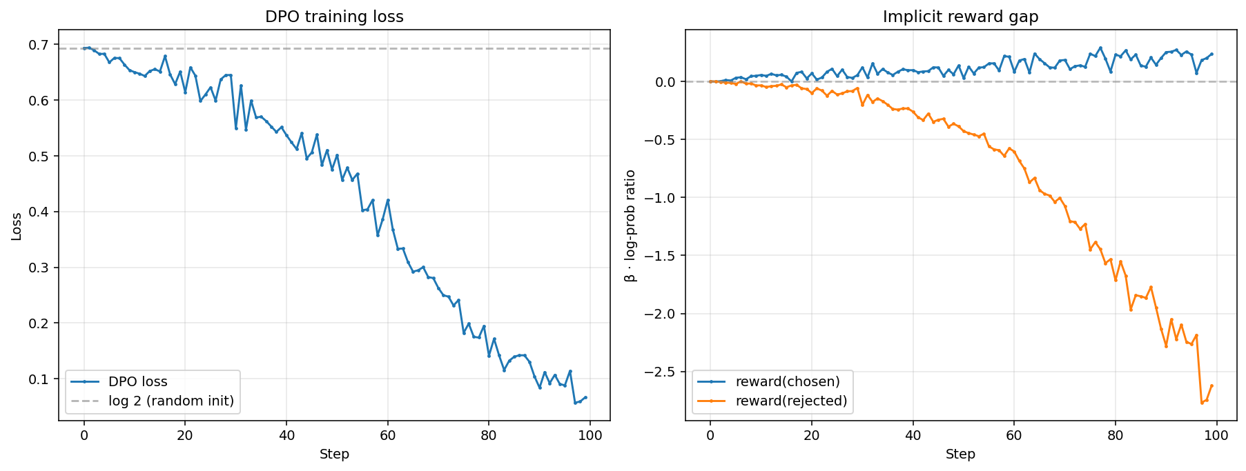
Figure 2: DPO training loss (left) and implicit reward gap (right) over 100 steps.
Left panel — DPO loss. Loss starts at 0.6931 (the random-init point, -log σ(0) = log 2 ≈ 0.6931) and falls steadily as the policy learns to prefer chosen over rejected. By step 99 it has dropped to about 0.07, an order of magnitude below random.
Right panel — implicit reward gap. The gap between reward(chosen) and reward(rejected) widens from 0.00 to about 2.86 over 100 steps. The chosen-response branch (blue) drifts slightly above zero, while the rejected-response branch (orange) is pushed strongly negative, producing the asymmetry DPO is designed for. This is the real diagnostic: if the reward gap did not widen, you would know something was wrong even if the loss looked fine.
DPO in production
For real LLM alignment, the trl (Transformer Reinforcement Learning, TRL) library wraps everything in a DPOTrainer class that mirrors the SFTTrainer we used in Part 8:
from trl import DPOTrainer, DPOConfig
from peft import LoraConfig, TaskType

lora_config = LoraConfig(
    r=16, lora_alpha=16,
    target_modules=["q_proj", "k_proj", "v_proj", "o_proj"],
    task_type=TaskType.CAUSAL_LM,
)

trainer = DPOTrainer(
    model=base_model,        # SFT-tuned model from Part 8
    ref_model=None,          # auto: use base with LoRA disabled as reference
    args=DPOConfig(
        output_dir="./dpo-out",
        beta=0.1,
        learning_rate=5e-6,  # much smaller than SFT's 2e-5
        max_length=512,
        max_prompt_length=256,
        gradient_checkpointing=True,
        per_device_train_batch_size=2,
    ),
    train_dataset=preference_dataset,   # columns: prompt, chosen, rejected
    tokenizer=tokenizer,
    peft_config=lora_config,
)
trainer.train()
When you pass peft_config, TRL uses the same base model with the LoRA adapter disabled as the reference π_ref, so no second model copy is needed. Combined with QLoRA-style 4-bit quantization and a small batch size, you can fit DPO on a 7B model on a single Kaggle T4 (T4 has 16 GB VRAM). That capability did not exist three years ago.
Note that the DPO learning rate is typically several times smaller than SFT, often 4-100× smaller depending on dataset size and beta (per TRL docs and the DPO paper community). The model is already well-aligned by SFT; DPO is making fine-grained adjustments, not relearning capabilities.
Alternatives to DPO
Several alignment methods address cases where DPO’s assumptions do not hold (for instance, when you lack a strong reference model or need stronger regularization):
| Method | Key idea | Advantage | Limitation |
|---|---|---|---|
| PPO/RLHF | RL with a reward model | Powerful, handles sequential rewards | Three model copies, on-policy rollouts, complex |
| DPO | Binary classification on log-prob ratios | Simple, offline (no rollouts needed) | Can be unstable at high learning rates |
| IPO (Azar et al., 2023) | Similar to DPO but with implicit regularization | More resistant to over-optimization | Slightly lower quality ceiling |
| ORPO (Hong et al., 2024) | Combines SFT + alignment in one loss | Single training stage | Newer, less battle-tested |
| SimPO (Meng et al., 2024) | Length-normalized log probs, no reference model | No reference model needed | Requires careful tuning |
DPO is among the most widely deployed as of 2026 because it is simple to implement, has good library support in TRL, and produces strong results on standard benchmarks.
Constructing preference data that actually teaches alignment
The quality of your preference dataset determines whether DPO produces a noticeably better model or just a slightly re-weighted one. A few practical guidelines:
Chosen and rejected should differ on the axis you care about. If you want the model to refuse harmful requests, your preference pairs should have a refusal as chosen and a helpful-but-harmful response as rejected, not just “longer vs shorter”. Vague quality differences produce weak alignment signals.
Avoid length bias. Human annotators consistently rate longer responses as higher quality even when they are not. A preference dataset collected from human raters without controls will teach the model to be verbose. Mitigate this by asking annotators to explicitly rate helpfulness independent of length, or by using a length-normalized reward signal like SimPO.
Margin matters. Prefer pairs where the quality gap between chosen and rejected is large and unambiguous. Borderline pairs (where annotators disagree or the difference is subtle) degrade training stability and produce noisy gradients. The beta parameter in the DPO loss controls how strongly the model is pushed away from the reference; pairs with low margin are better handled by higher beta (more conservative alignment).
Sample from your own model when possible. If you have an SFT model, generate multiple completions per prompt and have annotators rank them. This “self-play” data is typically more useful than human-written pairs because the rejected completions are close to your model’s actual distribution, which is where the alignment needs to happen.
Minimum viable dataset size: 1,000–5,000 preference pairs for a targeted behavior change (e.g., format consistency, refusal policy). Broad alignment (human preference across many dimensions) benefits from 10K–100K pairs as used in Anthropic’s or OpenAI’s alignment work.
Tuning beta and verifying the alignment is working
beta controls how far the model is allowed to deviate from the reference policy:
- Low
beta(0.01–0.05): Strong alignment pressure. The model moves aggressively toward chosen completions. Risk: the model may “over-align” and sacrifice quality on prompts not well-represented in the preference data. - High
beta(0.5–1.0): Conservative alignment. Stays close to the SFT reference. Risk: the alignment signal is too weak to change behavior noticeably. - Default
beta=0.1: The TRL default, works well for most cases.
Two diagnostics to run after every DPO training run:
1. Check the reward gap. Log chosen_reward - rejected_reward during training. It should increase monotonically. If it plateaus early or never rises above ~0.1, the model is not learning the preference signal; try a lower beta or more data.
2. Generate and compare samples. Pick 10–20 representative prompts. Generate completions from the SFT model (reference) and the DPO model side-by-side. Human-evaluate which is better. A correctly trained DPO model should show clear quality improvements on the axes your preference data targeted, with no degradation on unrelated axes.
import torch
from transformers import AutoModelForCausalLM, AutoTokenizer

def generate(model, tok, prompt, max_new=100):
    ids = tok.apply_chat_template(
        [{"role": "user", "content": prompt}],
        return_tensors="pt", add_generation_prompt=True
    )
    with torch.no_grad():
        out = model.generate(ids, max_new_tokens=max_new, do_sample=False,
                              pad_token_id=tok.eos_token_id)
    return tok.decode(out[0, ids.shape[1]:], skip_special_tokens=True)

prompts = [
    "Explain the difference between precision and recall.",
    "Write a one-paragraph cover letter for a data scientist role.",
]

for p in prompts:
    print(f"Prompt: {p}")
    print(f"  SFT : {generate(sft_model, tokenizer, p)}")
    print(f"  DPO : {generate(dpo_model, tokenizer, p)}")
    print()
If your DPO model consistently produces better answers on the targeted behavior and no worse answers on unrelated prompts, the alignment run succeeded.
What you’ve now built
You started in Part 1 by turning raw text into vectors, the foundational act that makes language manipulable by calculus. Parts 2 through 6 built every piece of the Transformer from scratch in PyTorch: the self-attention mechanism that lets tokens communicate across arbitrary distances, multi-head attention that runs several attention patterns in parallel, positional encoding that restores the sequence order that attention discards, and the full encoder-decoder stack that ties everything together. Every equation in those parts has a concrete, runnable Python counterpart you built yourself.
Part 7 bridged theory to practice: you loaded a real pre-trained LLM with the Hugging Face APIs and saw how tokenization, special tokens, and chat templates work in production. Part 8 ran a full Supervised Fine-Tuning loop (watching the loss drop roughly two orders of magnitude) and measured what SFT costs in memory, establishing the wall that stops single-GPU fine-tuning at the 7B scale. Part 9 broke through that wall with LoRA and QLoRA, shrinking trainable parameters from 100% to under 1% while preserving nearly all of the quality. And in this part you closed the loop with DPO, replacing the three-stage PPO/RLHF pipeline with a single binary classification loss that teaches the model which valid responses to prefer.
You now possess the same conceptual toolkit that every modern AI lab uses to build LLMs. GPT-4, Claude, Gemini, and every other state-of-the-art model is built on these exact foundations; the difference is scale, not concept. The interesting questions from here are no longer architectural: they are about what to train on, how to evaluate at scale, how to deploy responsibly, and how to align with goals that shift over time. Those are the open questions for the next decade, and you are now equipped to engage with them seriously.
Thank you for reading the whole series.